by Edwin X Berry, PhD, Theoretical Physics, CCM
Ed Berry LLC, Bigfork, Montana
To read key referenced papers:
- CO2 Coalition paper
- Dia Ato paper
- Bernard Robbins paper
- Eike Roth paper
Click here
Responsiveness of Atmospheric CO2 to Fossil Fuel Emissins
by Jamal Munshi
Ferdinand Engelbeen says Jamal Munshi has not proved absence of correlation.
What do you think? Add your comment below.
A Thermal Acid Calcification Cause for Seasonal Oscillations in the Increasing Keeling Curve
Download this Excel file here: https://edberry.com/Excel-File
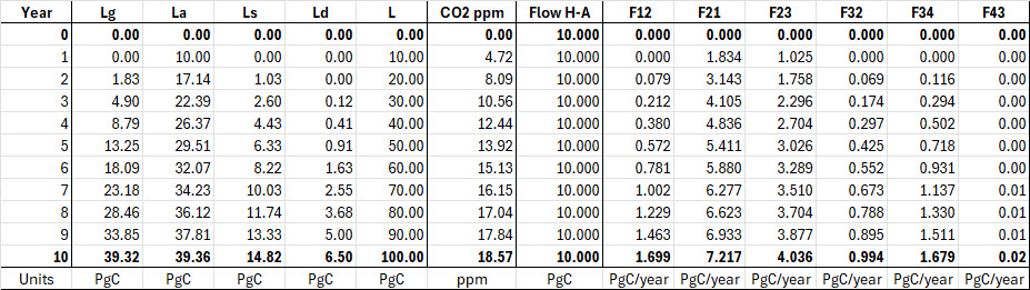
Here is table “Berry Carbon Flow Test” for discussion in our comments.
I request Ferdinand and anyone else who is contesting my calcuations to present your calculations for comparison.
We assume that the natural carbon cycle is at constant levels as shown in Figure 3.
With that information, we insert human carbon into the atmosphere at a constant rate of 10 PgC per year. Then we calculate annual time steps to see how much human carbon ends up in each reservoir each year.
This simple calculation is a way to compare our calculations because we keep human carbon inflow constant for each year.
The years run from zero to ten. All the L data are in PgC, and flow data are in PgC/Year.
Lg = land, La = atmosphere, Ls = surface ocean, Ld = deep ocean, L is the total PgC in the carbon cycle for each year. Ntice L increases by 10 PgC each year.
The CO2 ppm column simply converts the PgC in La to ppm.
Here’s how it works.
Year 0: 10 PgC is added to La, but you don’t see it until the beginning of Year 1.
Year 1: the 10 PgC in La produces outflows to Lg and Ls. We see the result in Year 2.
Year 2: the outflows from La have moved some carbon to Lg and Ls. Etc.
Notice that as La gets more PgC, its Outflow to Lg and Ls increase, etc.
While La increased by 7.14 PgC from Year 1 to Year 2, it increased by only 1.49 PgC from Year 9 to Year 10.
Also notice that as Lg and Ls get more carbon, they send carbon back to La.
Adjustment, Residence, E-time Compared
IPCC’s response times fail physics
Physics e-time has a precise definition. The IPCC times do not. In summary:
- Physics: e-time is the time for the level to move (1 – 1/e) of the distance to its balance level.
- IPCC: adjustment time is the time for the level to “substantially recover” from a perturbation.
- IPCC: residence time is the average time a CO2 molecule stays in the atmosphere.
IPCC defines “adjustment time (Ta)” as:
The time-scale characterising the decay of an instantaneous pulse input into the reservoir.
Cawley defines “adjustment time (Ta)” as:
The time taken for the atmospheric CO2 concentration to substantially recover towards its original concentration following a perturbation.
The word “substantially” is imprecise.
Cawley follows IPCC to define “residence time (Tr)” as:
The average length of time a molecule of CO2 remains in the atmosphere before being taken up by the oceans or terrestrial biosphere.
In summary, IPCC uses two different response times where it should use only e-time:
- When the level is far from its balance level (which can be zero), IPCC thinks e-time is an adjustment time because the level is moving rapidly toward its balance level.
- When the level is close to its balance level, IPCC thinks e-time is a residence time because “molecules” are flowing in and out with little change in level.
Figure A illustrates how e-time relates to IPCC’s adjustment and residence times.
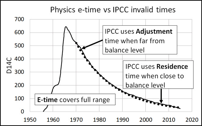
Figure A. E-time covers the full range of movement of level to a balance level. IPCC adjustment and residence times apply to only each end of the range.
IPCC, 2001: Working Group 1: The scientific basis. Appendix 1 – Glossary.
Lifetime
Lifetime is a general term used for various time-scales characterising the rate of processes affecting the concentration of trace gases. The following lifetimes may be distinguished:
Turnover time (T) is the ratio of the mass M of a reservoir (e.g., a gaseous compound in the atmosphere) and the total rate of removal S from the reservoir: T = M/S. For each removal process separate turnover times can be defined.
Adjustment time or response time (Ta) is the time-scale characterising the decay of an instantaneous pulse input into the reservoir. The term adjustment time is also used to characterise the adjustment of the mass of a reservoir following a step change in the source strength.
Half-life or decay constant is used to quantify a first-order exponential decay process.
The term lifetime is sometimes used, for simplicity, as a surrogate for adjustment time.
In simple cases, where the global removal of the compound is directly proportional to the total mass of the reservoir, the adjustment time equals the turnover time: T = Ta.
In more complicated cases, where several reservoirs are involved or where the removal is not proportional to the total mass, the equality T = Ta no longer holds.
→Carbon dioxide (CO2) is an extreme example. Its turnover time is only about 4 years because of the rapid exchange between atmosphere and the ocean and terrestrial biota.
However, a large part of that CO2 is returned to the atmosphere within a few years.
Thus, the adjustment time of CO2 in the atmosphere is actually determined by the rate of removal of carbon from the surface layer of the oceans into its deeper layers.
Although an approximate value of 100 years may be given for the adjustment time of CO2 in the atmosphere, the actual adjustment is faster initially and slower later on.
Ed,
1.You have not been able to tell me how natural processes that remove more carbon from the atmosphere than they add, are nevertheless are responsible for CO2 growth.
2. We agree that there is little of your “human carbon” in the present atmosphere. I have told you why: the dilution of the Seuss Effect, known about since the 1950’s. You have not responded.
I have several times judged high school debates. When one debater ducks question from the other, that debater loses. You lose, Ed.
David Andrews July 16, 2025 at 9:33 am
Dear David,
That is one of the most complicated pseudo explanations of a simple concept I may have read.
First, you have no formula for adjustment time, so it is meaningless in the context of this discussion. It has no bearing on how to calculate or explain the evolution of the carbon cycle. It is a diversion from physics.
Second, the only meaningful time constant is e-time because it has a real formula that predicts things and applies universally to our discusion.
Third, for a simple explanation of how carbon flows in IPCC’s carbon cycle model, see my Figure 7. The top row illustrates IPCC’s natural carbon cycle at equilibrium. Change the numbers if you wish but every set of suggested numbers will have an equilibium distribution. This is the condition where the carbon flows between the boxes are equal.
The second row in Figure 7 illustrates human carbon at equilibrium if all human emissions ended. The human carbon cycle will have the same percentages in each box as the natural conbon cycle because of the climate equivalent principle.
Figure 7 shows human carbon left in the atmosphere at equilibrium is about 4 ppm when human carbon has added about one percent to the carbon in the natural carbon cycle.
Such equilibrium represents a maximum entropy for the carbon cycle.
Figure 7 shows what happens to human carbon that we introduce into the atmosphere. The addition of human carbon to the atmosphere begins in a low entropy condition. Human carbon will flow to the other boxes in a manner that increases the entropy as fast as possible.
Human carbon cannot increase the CO2 level in a manner that would lower the entropy of either the human carbon cycle or the natural carbon cycle.
The CO2 Coalition’s argument that human carbon causes all the CO2 increase, or somehow causes the natural carbon cycle to cause the CO2 increase fail because they lower the entropy of the total carbon cycle, which is an impossible.
David Andrews July 16, 2025 at 9:55 am
“1.You have not been able to tell me how natural processes that remove more carbon from the atmosphere than they add, are nevertheless are responsible for CO2 growth.”
Your question itself shows you do not understand the physics of the carbon cycle. Even in my last comment, I explained the basics of how human carbon affects the carbon cycle.
“2. We agree that there is little of your “human carbon” in the present atmosphere. I have told you why: the dilution of the Seuss Effect, known about since the 1950’s. You have not responded.”
Read my draft paper above.
First, we disagree WHY human carbon is a small part of the present atmosphere. You claim it is because natural carbon atoms “replaced” human carbon atoms in the atmosphere. Your explanation defies physics and would decrease the entropy if it happened.
Second, the Seuss effect is a calculated effect, not a cause. It does not even deserve a special name but you make a big deal of it because you incorrectly believe it somehow strengthens your argument. It does not.
The D14C data show human carbon has lowered the D14C level by less than 8%. That proves human carbon is less than 8% of the atmosphere.
This D14C “dilution” is a result of the continuing inflows of human carbon and natural carbon into the atmosphere. These inflows set balance levels. The dilution is a measure of the human carbon balance level compared to the natural carbon balance level. Period.
At the risk of sounding silly (I’m an old land surveyor who’s expertise is in knowing what to measure and mostly at sea on the technicalities in this discussion) I will ask if the mass of the atmosphere is constant? It seems that the mass balance approach assumes that it is but Dr. Ed’s approach does not. I know that lots of atmospheric gasses are added and removed by natural and anthropogenic processes.
DMA,
A better name for the argument often called “mass balance” is simply “carbon conservation.” If human emissions put 100 units/yr of carbon into the atmosphere, but the measured carbon growth rate is only 45 units/yr, then by carbon conservation, natural processes must be removing 55 units/yr and putting it in somewhere else. The carbon can’t just evaporate. These are good average numbers. Ed is trying to convince you that these same natural processes are somehow adding carbon to the atmosphere, but he never directly tells us how. That is because they are not.
Ferdinand,
“Output of the atmosphere is NOT proportional to the absolute CO2 pressure, but proportional to what Henry’s law dictates for the ocean surface. Not that it makes much difference, as input – output is a meager 5 PgC/year (~2.5 ppmv/year) at a level of 900 PgC in the atmosphere. For the absolute output that makes some 16 PgC/year. That is all. All the rest of the 200 PgC/year is what other processes absorb and bring back and these processes are largely independent of the CO2 pressure in the atmosphere. Like the uptake by vegetation in spring/summer: 120 PgC/half year only from the sun and temperature. The net effect of the full biological cycle is only 2.5 PgC/year more out than in.”
You and David keep repeating stuff that has no scientific basis. That is not Henry’s Law. You know it is not Henry’s Law. I’ve shown you that it is not Henry’s Law, but you continue to insist it is Henry’s Law. Read any Chemistry 101 textbook and it will recite Henry’s Law exactly like I have stated. Dr. Ed showed in his first paper that C14 bomb data supports his hypothesis, L/Te = outflow. How is it possible to debate people who refuse to accept natural law? You don’t accept the Equivalence Principle. You don’t accept the gas laws. You don’t accept scientific method. You refuse to answer my questions. You and David are so chained to your beliefs that you can’t accept that they are wrong.
David Andrews
Aren’t the units computed as a percentage of the atmosphere? If that mass is changing the units aren’t the same. Human emissions are tons of CO2 but total CO2 is in tons computed by multiplying a measured percentage times a figure that maybe not constant.
Ferdinand,
So, for input=output, Tau has no meaning then what is Te?
David Andrews July 16, 2025 at 11:27 am
David,
There you go again:
“… then by carbon conservation, natural processes must be removing 55 units/yr and putting it in somewhere else.”
You have physics backwards. “Natural processes” don’t “remove” human carbon from the atmosphere, like a dump truck removes garbage.
Human carbon flows out of the atmosphere toward its equilibrium distribution in the carbon cycle, thereby increasing its entropy.
Simple calculations based upon human emissions and reasonable Te for the six flow nodes, show human CO2 cannot cause all, or even most, of the CO2 increase because human carbon added to the atmosphere flows to the other boxes too fast to allow human CO2 to cause all the CO2 increase.
You are trying to tell people that human emissions cause all the increase in the face of carbon cycle data, including D14C data, that prove your claim is impossible.
I don’t need to prove how nature would cause the CO2 increase. You need to prove that human CO2 caused the increase.
Science requires we use the null hypothesis which says all changes are natural until proven otherwise. The burden of proof is on you to prove otherwise.
You have not and cannot do that.
Stephen Paul Anderson, July 16, 2025 at 11:40 am
Stephen. if the ocean surface in average, per Henry’s law, is in equilibrium with the atmosphere, that is when in average there is a fixed ratio between CO2 in the atmosphere and the ocean surface waters, then still a lot of CO2 can be exchanged, because some parts (near the equator) are warmer, thus release CO2 and some parts are colder, thus absorb CO2. That is called a dynamic equilibrium. CO2 is removed near the poles and that sinks with the cold waters into the deep oceans, to return some 1,000 years later near the equator, releasing its CO2 again.
At that moment there still is a
Te(a-d) = 589 PgC / 25 PgC/year = 23 years.
For the reverse flow:
Te(d-a) = 37,100 PgC / 25 PgC/year = 1,484 years.
Tau is not calculable as (input = output) and division by zero is not possible.
There is no usable information in Te(a-d) or Te(d-a), as the only point of interest is if the input and output flows are equal and neither of these two gives us that information.
In the current atmosphere the CO2 mass is already 900 PgC which makes that the outflows (and also inflows) into the deep oceans increased (let us assume in ratio, thus + 50%):
Te(a-d) = 900 PgC / 40 PgC/year = 22.5 years
Te(d-a) = 37,100 PgC / 40 PgC/year = 928 years
The output from the atmosphere to the deep oceans increased in ratio, thus Te(a-d) remained about the same, but as the carbon content of the deep oceans hardly changed, Te(d-a) did change a lot.
Again, that doesn’t give the slightest information of the actual change of CO2 in the atmosphere or deep oceans.
What happened to Tau? Yet it is calculable: the estimated net sink rate from the atmosphere into the deep oceans (input – output) is 2.0 PgC/year. That gives for Tau:
Tau(a-d) = (900 – 589) PgC / 2 PgC/year = 155 years
If Tau doesn’t change over time, which is the case for a linear decay, then we can calculate the carbon increase or decrease in the atmosphere, ocean surface, deep oceans and vegetation for the past and the future – if human emissions and temperature are known…
Tau gives us usable information, Te doesn’t.
Dr. Ed, July 16, 2025 at 11:58 am
“Simple calculations based upon human emissions and reasonable Te for the six flow nodes, show human CO2 cannot cause all, or even most, of the CO2 increase because human carbon added to the atmosphere flows to the other boxes too fast to allow human CO2 to cause all the CO2 increase.”
Simple calculation indeed shows that human FF is readily distributed over all reservoirs, which all increase in carbon content. But as human emissions (according to your Te’s) are fast getting out of the atmosphere, where is the rest of the observed increase in the atmosphere coming from?
Something doesn’t add up in your carbon mass balance…
Ferdinand Engelbeen
July 16, 2025 at 7:13 am
I know your mind is made up, but humor me while I try to understand your interpretation of F = k•s•ΔCO2.
Do you agree that output from the atmosphere is equivalent to – dCO2/dt, where CO2 is the concentration of CO2 in the atmosphere (the minus sign indicates output is reducing CO2)?
Second, by splitting Feely’s equation, do you agree that F- = k*p(CO2) = – dCO2/dt?
Also, that F+ = k * s * pCO2(aq) = + dCO2/dt?
Finally, at equilibrium, although there is no net transfer, do those forward and reverse rate equations still apply?
Ferdinand Engelbeen July 16, 2025 at 1:04 pm
Since human CO2 can’t cause all the CO2 increase, the only other possibility is natural CO2 increased.
However, I don’t need to show or prove how nature is doing that.
(This is somewhat like an astromoner finding something is causing a planet to deviate from its expected orbit. The astronomer does not have to find WHAT is causing the deviation in order to prove his calculations are correct. Typically, someone else finds the cause.)
Science requires we use the null hypothesis which says all changes are natural until proven otherwise. The burden of proof is on you to prove that my calculations are wrong or the numbers I use are wrong.
Ferdinand,
So, Te = L/outflow=589PgC/25PgC/yr=23.6 years. Where did you get your outflow from?
Ferdinand,
Also, what Te(c) vs. Te(a-d)?
DMA
July 16, 2025 at 11:05 am
July 16, 2025 at 11:45 am
Although there are gasses entering and exiting the atmosphere, their concentrations remain relatively constant except CO2 which has been gradually increasing. Fortunately, we have the Mauna Loa and other places monitoring it. It’s more difficult to measure CO2 in other reservoirs. The mass balance has to do with where the fossil fuel carbon went. I have no idea why David Andrews doesn’t see the obvious that whatever is no longer in the atmosphere is somewhere distributed between the other reservoirs. The hard part is what Dr. Ed did, to use estimates of reservoir content and mass transfer rates to figure out what went where when. David Andrews’ simple math is insufficient to explain all the data correctly using the correct physical principles involved.
“Aren’t the units computed as a percentage of the atmosphere?”
That’s a good question. The volume of the atmosphere is constant and the mass is easily determined by C * V. Ocean concentrations are measured, but the volumes vary widely and it’s impossible to know concentrations and volumes of the land.
That’s why Dr Ed’s methods are so useful. It allows a way to evaluate the estimates and synchronize them with the known values which are mainly just the changing concentration of CO2 in the atmosphere. If there’s any missing carbon, you can be sure to find it somewhere in a tree or on the ocean floor.
David Andrews
July 16, 2025 at 9:33 am
I will just add two things to Dr. Ed’s answer at July 16, 2025 at 10:16 am. First, the long 50-year Tau is an artifact of using the preindustrial value of CO2 as the equilibrium concentration if net zero ever happened. Because of bioexpansion, the new equilibrium will be at a much larger CO2 value.
Second, yes, I postulated “exponentially” growing natural emissions to keep up with the Mauna Loa curve using an e-time of about four years. I also tried no change in natural emissions and postulated slowly increasing e-time to maintain the agreement with Mauna Loa data. But that required deviating greatly from the universally accepted constant e-time of about 4 years. I couldn’t make it correlate with both constant natural emissions and constant e-time. Can you demonstrate a scenario matching Mauna Loa data using a 4-year e-time without increasing natural emissions?
Ed,
Must I go back to your old papers and identify plots which show human emissions greater than atmospheric accumulation? The world understands: those plots mean net global uptake has consistently been positive. The world understands: that proves natural processes are removing net carbon from the atmosphere. The world understands: that proves human emissions cause the CO2 rise. A dump truck analogy works. Nine dump truck loads move carbon from land/sea reservoirs to the atmosphere. Ten dump truck loads move carbon from the atmosphere to land/sea reservoirs. As a result, natural processes mitigate the increase in atmospheric carbon that humans cause. You know the consistently positive net global uptake falsifies your false theory and that makes you panic.
Please don’t repeat that your calculation shows only a small “human carbon” component in the present atmosphere. That is a correct conclusion in line with mainstream science, anticipated 70 years ago, and not particularly important.
Entropy??? Careful Mr. Ed, I taught thermodynamics. Go ahead, pursue this line. Make my day.
Jim,
“universally accepted constant e-time of about 4 years. ” (?!)
…universally accepted by novices that don’t understand the difference between adjustment time and residence time perhaps. So you really think the time constant for surface ocean/ deep ocean mixing is four years? Or do you think that particular mixing time is irrelevant? Can you tell me where I referenced the 1750 equilibrium in my little exercise? You are not making much sense. Explain yourself.
Jim,
I just noticed your comments about the growth in carbon in the ocean (“acidification”) and in the biosphere (the greening that the CO2 coalition talks about.) Of course that results from natural processes moving carbon out of the atmosphere and into those reservoirs. It is where the net global uptake went. What I don’t understand is why you apparently think that supports the wrong notion that natural processes cause the atospheric increase.
Ferdinand,
“Observed: 5 PgC/year = 10 PgC/year + natural inputs – natural outputs
Or natural outputs are 5 PgC/year larger than the natural inputs.
Even if the natural outputs include half the human input of 5 PgC/year human supplied FF molecules, then still the full increase of 5 PgC/year in the atmosphere is caused by the human emissions.
According to your ideas, natural outputs are smaller than natural inputs.
Who is violating the carbon mass balance ánd the equivalency principle here?”
You. You are violating the carbon mass balance and the equivalence principle. You flunk Physics 101. Let me help you.
dCO2/dt = Inflow – Outflow
Inflow=Lb/Te (Lb=Balance Level)
Outflow= L/Te
L=430ppm
If we use dC/dt=2ppm/yr (4.24PgC/yr) and a Te of 4 years from Dr. Ed’s paper.
Outflow=430ppm/4yr=107.5 ppm/yr
Inflow= 107.5ppm/yr+ 2ppm/yr =109.5ppm/yr
Balance Level = 109.5ppm/yr(4yr)=438ppm
Te (eTime) is the time it takes for Level to reach 0.693 the distance from the level to the balance level. So, in 4 years from now, the level should be 435.54ppm.
If inflow is 5ppm human and 104.5ppm natural, then in 4 years when the level is 435.5ppm, human CO2 can be no more than 20ppm of the total. Outflow, which is 107.5ppm/yr, is 4.945ppm/yr human and 102.555ppm/yr natural. So, of the 2ppm/yr increase, 0.055ppm is human and 1.945ppm is natural. Natural emissions are greater than natural sinks. This is conservation of mass and in compliance with the equivalence principle.
David,
Dr. Ed has talked about adjustment time. Te is the time it takes for level to go 0.693 the distance to the balance level. So, in 4 years it will be at 435.5ppm. In 8 years it will be at 437.2 ppm. In 12 years it will be at 438ppm. So, some of the CO2 molecules have very short residence times and some have long residence times. It takes 3 or 4 Te’s to reach the balance level. (Actually, it never does. That is the nature of Euler’s number.) Residence time has nothing to do with the mathematics of the conservation of mass of carbon in the atmosphere.
Ferdinand,
P.S.-This is the solution to the first order linear differential equation. There is no other solution.
Stephen P Anderson, July 16, 2025 at 11:56 pm
“dCO2/dt = Inflow – Outflow
Outflow= L/Te
L=430ppm”
So far so good. Then:
“Inflow=Lb/Te (Lb=Balance Level)”
Say what? Are you saying that soil bacteria which remove plant rests and humans, which exhale 40,000 ppmv CO2 do that in ratio with CO2 in the atmosphere?
“If we use dC/dt=2ppm/yr (4.24PgC/yr) and a Te of 4 years from Dr. Ed’s paper.
Outflow=430ppm/4yr=107.5 ppm/yr
Inflow= 107.5ppm/yr+ 2ppm/yr =109.5ppm/yr
Balance Level = 109.5ppm/yr(4yr)=438ppm”
There it goes completely wrong.
Te has nothing to do with the decay rate of any extra injection of CO2, from whatever source.
Te = mass / output.
Between 1750 and current, both mass and output may have increased with 50% (which is not the case, outputs did increase more slowly), leaving a rather constant (or increasing) Te.
Between 1958 and 2025 dCO2/dt increased a five fold from 0.5 ppmv/year to 2.5 ppmv/year.
Simply said: Te and dC/dt have nothing in common and the 4 years residence time and the real decay rate or adjustment time (Tau) are completely different items.
Why is that? Because most of the outflows are (near) completely independent of the absolute CO2 pressure in the atmosphere. These are temperature, sunlight, bacterial and other biological processes, independent of how much CO2 resides in the atmosphere.
The height of the inflows and outflows has zero impact on the decay rate of CO2 in the atmosphere, only the difference counts: dCO2/dt = inflows – outflows.
dCO2/dt is quite exactly known, outflows only roughly, thus Te is even far from certain.
Then the balance level: that can be back calculated from the level in the atmosphere and the resulting dCO2/dt. Where dCO2/dt = 0, that is the balance level:
https://sealevel.info/Global_Carbon_Budget_2023v1.1_with_removal_rate_plot2.png
Between 280 and 300 ppmv.
“Te (eTime) is the time it takes for Level to reach 0.693 the distance from the level to the balance level. So, in 4 years from now, the level should be 435.54ppm.”
Te is level / output, that “can” be like Tau, the time to reach 1/e of the balance level, if and only if all inflows, container and outflows are unidirectional. That is the “lake / container / bath tube” model. Then Tau is smaller than to equals Te.
If there are back flows, which is the case for 95% of all CO2 flows the real world, then Te and Tau are decoupled and completely independent of each other. That is the “fountain” model, where lots of CO2 are pumped in and out, without any influence on the quantity that is really removed.
The calculated Tau, based on the current 420 ppmv and the calculated balance level of around 290 ppmv and the observed dCO2/dt of 2.5 ppmv/year gets:
Tau = (420 – 290) / 2.5 = 52 years
“So, of the 2ppm/yr increase, 0.055ppm is human and 1.945ppm is natural. Natural emissions are greater than natural sinks. This is conservation of mass and in compliance with the equivalence principle.”
One little problem: the CO2 level, both in the oceans and the biosphere increased with in total about 1 ppmv/yr as mass. Both oceans and biosphere together supplied near 2 ppmv/yr to the atmosphere.
Total increase in all containers together: 3 ppmv/year, with an external (human) supply of 2 ppmv/year. Something doesn’t add up here…
Moreover, with 1% to 5% in the input (1958-current) the observed FF level in the atmosphere is already over 10% and in the ocean surface over 6%… With your calculation that would be less than 1%.
Stephen P Anderson, July 17, 2025 at 12:13 am
“Te is the time it takes for level to go 0.693 the distance to the balance level.”
That is the essence of the discussion here:
Te is NOT the time it takes to decay to the balance level. That is Tau.
Te in this real world has nothing to do with reaching a balance level, it only shows how long an individual CO2 molecule “resides” in the atmosphere, before being removed (with a change in mass) or replaced (without a change in mass) out of the atmosphere. Only 2.5% of CO2 mass is removed per year, while 25% per year is replaced.
Or a difference between 50 years for Tau and 4 years for Te.
David Andrews
July 16, 2025 at 9:38 pm
I can’t immediately tell you what the time constant for surface to deep ocean is, but I’m sure I can get it from Dr. Ed’s paper. It will be different because of the concentration and volume differences. The important point to note is that not all the atmosphere carbon going to the surface is removed to the deep. There is a gradual increase in CO2 there as well, which contributes to the excess CO2 increasing in the atmosphere.
Truck load analogies are not compatible with physical processes. Stick to Magic Math.
July 16, 2025 at 9:50 pm
Better yet, graduate to step-wise integration and compartment modelling. Then you will see for yourself how natural emissions and FF both contribute to atmospheric increase.
Ferdinand,
“Why is that? Because most of the outflows are (near) completely independent of the absolute CO2 pressure in the atmosphere. These are temperature, sunlight, bacterial and other biological processes, independent of how much CO2 resides in the atmosphere.”
Dr. Ed’s hypothesis is based on Henry’s Law, the Ideal Gas Law, and correlates well with C14 bomb data. Te is e folding time which comes from the solution of the differential equation. Your Tau is a mathematical construct. It does not come from the solution of the conservation of mass equation, and it has no basis in math or physics. Its basis is a desired outcome. Dr. Ed’s model is beautifully simplistic and violates no natural laws. Your’s isn’t. Dr. Ed’s solution comes straight from the textbooks that I studied. Your’s does not. Your Tau violates the Equivalence Principle and treats human CO2 and natural CO2 differently. As long as you insist that non-science and non-logic are your basis, we are at an impasse.
Sorry but I have to stop here…
I need to make a presentation for a direct confrontation with Hermann Harde about the same subject for the Scandinavian Skeptics conference and need to transfer all my data to a new computer (thanks to Microsoft, which made Windows 11 not compatible with my only 7 years “old” model), my 3D-printer got broken and I just sold my brand new solar panels that I didn’t use, because of the perfidious change in tariffs they will imply when installed.
Still will finish the A-B item and the Berry challenge within a few days I hope, as promised.
David,
Jim,
“universally accepted constant e-time of about 4 years. ” (?!)
“…universally accepted by novices that don’t understand the difference between adjustment time and residence time perhaps. So you really think the time constant for surface ocean/ deep ocean mixing is four years? Or do you think that particular mixing time is irrelevant? Can you tell me where I referenced the 1750 equilibrium in my little exercise? You are not making much sense. Explain yourself.”
4 years is the universally accepted eTime for outflow from the atmosphere. If you would read Dr. Ed’s paper he says that the eTime for surface ocean to deep ocean is different. I thought we were all talking about atmospheric carbon? The eTime for atmosphere to land will be different than atmosphere to surface ocean, but total eTime is faster than the fastest individual eTime. That’s why the Bern Model is wrong. Thus, we get an overall eTime of 3.5 to 4 years.
Ferdinand,
“One little problem: the CO2 level, both in the oceans and the biosphere increased with in total about 1 ppmv/yr as mass. Both oceans and biosphere together supplied near 2 ppmv/yr to the atmosphere.
Total increase in all containers together: 3 ppmv/year, with an external (human) supply of 2 ppmv/year. Something doesn’t add up here…
Moreover, with 1% to 5% in the input (1958-current) the observed FF level in the atmosphere is already over 10% and in the ocean surface over 6%… With your calculation that would be less than 1%.”
Show your evidence.
David Andrews July 16, 2025 at 9:34 pm
Gee, David, I’m really scared. You may have taught thermodynics but that does not mean you KNOW thermodynamics.
So, challenge me on my comments above about entropy.
Jim,
You have not given us much information about your spreadsheet but assert various conclusions. Some of your comments make me wonder whether it is constrained by carbon conservation. For example “There is a gradual increase in CO2 [in the surface ocean] as well, which contributes to the excess CO2 increasing in the atmosphere.” I imagine your spreadsheet has a row for each year, and columns showing carbon stocks in different places. If you sum all the stocks in a row (year), how does that sum vary year to year?
My other main question about your analysis is one asked before but neither you nor Ed nor anyone else has responded. When you say “Then you will see for yourself how natural emissions and FF both contribute to atmospheric increase” are you simply saying that the present atmosphere contains only a small quantity of “human carbon”? You should know what I think of that argument.
Stephen,
A last comment:
Dr. Ed’s hypothesis is based on Henry’s Law, the Ideal Gas Law, and correlates well with C14 bomb data.
Dr. Ed’s hypothesis should be based on Henry’s Law, which implies a current equilibrium between atmosphere and average ocean surface of 295 ppmv for the current average sea surface temperature. Not 438 ppmv, according to your calculation, which is based on a Te of 4 years only, not the real, calculated from observations, decay rate of 50 years:
https://www.ferdinand-engelbeen.be/klimaat/klim_img/acc_decay.png
Where A are the FF emissions, observed increase in the atmosphere, the influence of temperature on the equilibrium pCO2 of the ocean surface since 1850, calculated with the formula of Takahashi and the resulting ΔpCO2 between atmosphere and ocean surface.
B is the observed net dCO2/dt with a polynomial to avoid the year by year variability, caused by T variability.
C is the resulting Tau, which is what shows the time to reach 1/e of the ΔpCO2.
The latter is based on every calculation of e-fold decay rates for any process in dynamic equilibrium where one of the components is changed.
https://en.wikipedia.org/wiki/Exponential_decay
Again Te is NOT the decay rate of CO2 to a new equilibrium. That is Tau. Te only shows how long a single CO2 molecule resides in the atmosphere, thus how much CO2 mass is moved through the atmosphere, not how much CO2 mass is REmoved…
And where do we make any differentiation between FF and other CO2? Once in the atmosphere, FF CO2 increases the total mass of the atmosphere with 5 ppmv/year and half that amount as total mass (not the FF CO2 alone) is removed out of the atmosphere. No matter its composition.
Berry’s solution violates the carbon mass balance, because of his use of the much too short residence time, which does not reflect the observed decay rate of about 50 years.
Stephen P Anderson, July 17, 2025 at 7:06 am
Net uptake by the biosphere, based on the oxygen balance and oceans as remaining difference:
https://tildesites.bowdoin.edu/~mbattle/papers_posters_and_talks/BenderGBC2005.pdf
“We find the average CO2 uptake by the ocean and the land biosphere was 1.7 ± 0.5 and 1.0 ± 0.6 GtC/yr
respectively”
Increase in the ocean surface, about 10% of the increase in the atmosphere:
https://tos.org/oceanography/assets/docs/27-1_bates.pdf
Figure 3 and Table 2.
Increase in the deep oceans: the remainder of the net sinks for dCO2/dt minus FF emissions.
Increase of FF in atmosphere and oceans:
https://agupubs.onlinelibrary.wiley.com/doi/full/10.1029/2001GC000264
Figure 4.
Based on the drop in 13C/12C ratio: over 10% FF in the atmosphere and over 6% in the ocean surface, calculated for a δ13C level of FF of -25 per mil and an atmosphere at average -6.4 per mil δ13C. Vegetation grows, thus with more CO2 uptake than release, which enriches the atmosphere in 13C at +24 per mil δ13C. Thus is not the cause of the enormous δ13C drop, not seen in the past 800,000 years, when δ13C levels were average -6,5 +/- 0.4 per mil, despite huge changes of 90 ppmv over glacial / interglacial transitions.
Ferdinand Engelbeen July 17, 2025 at 7:38 am
Dear Ferdinand,
You wrote, “Berry’s solution violates the carbon mass balance, because of his use of the much too short residence time, which does not reflect the observed decay rate of about 50 years.”
That is not true because my model begins with the Continuity Equation (1), which ensures my model conserves carbon mass. This conservation is entirely independent of Te.
This negates everything you claimed in your comment because you have based your claims on your fiction about my model.
Your model does not conserve carbon because (a) you have no continuity equation that forces conservation of carbon mass and (b) my Section 3.1, equations (10) and (11) show the critical error in your carbon mass balance equation.
Ferdinand.
“Dr. Ed’s hypothesis should be based on Henry’s Law, which implies a current equilibrium between atmosphere and average ocean surface of 295 ppmv for the current average sea surface temperature. Not 438 ppmv, according to your calculation, which is based on a Te of 4 years only, not the real, calculated from observations, decay rate of 50 years:
https://www.ferdinand-engelbeen.be/klimaat/klim_img/acc_decay.png
Where A are the FF emissions, observed increase in the atmosphere, the influence of temperature on the equilibrium pCO2 of the ocean surface since 1850, calculated with the formula of Takahashi and the resulting ΔpCO2 between atmosphere and ocean surface.”
It is based on Henry’s Law and the Ideal Gas Law. Henry’s Law doesn’t imply what you say it implies. Your’s and Takahashi’s ΔpCO2 is not part of Henry’s Law. If you keep repeating it is, I’ll keep repeating it isn’t.
Ferdinand,
Is the Scandinavian Skeptic’s Conference in English and is it going to be recorded?
Dr. Ed, July 17, 2025 at 8:18 am
dL / dt = Inflow – Outflow (1)
Agreed
Outflow = L / Te (2)
Upside down…
Te = L / outflow but you may only reverse that formula if, and ONLY if, all flows are unidirectional from input via the container to the output.
How do you calculate the 60 ppmv/year in spring/summer into vegetation with that formula, when the outflow goes from near zero to maximum in a few months, even lowering the L in the atmosphere?
Lb = Inflow * Te (4)
Completely wrong: Lb is not set by the inflows, it is set by the equilibrium between ocean surface and atmosphere per Henry’s law at current SST, that is about 295 ppmv.
Again your formula is true if, and ONLY if, all flows are unidirectional, or the “lake/container/bath tube” model. Not applicable at all for the real world, where 95% of all CO2 flows are just cycling in and out the atmosphere.
Further, one can threat the human and natural flows apart, but that makes no sense at all, as once the human FF is added to the atmosphere, its mass is there for 100% and only can be removed as mass, not apart as “human” and “natural” CO2, even if it is possible to do that.
Sorry I have to go now, I did make some example of how FF accumulates in the atmosphere, but that is somewhere at the beginning of this discussion…
Stephen P. Anderson, July 17, 2025 at 8:36 am
Takahashi’s formula IS the change in ratio of CO2 between atmosphere and ocean waters per Henry’s Law. That is the change in solubility of CO2 in seawater with temperature of about 4%/°C. That is all. Not over 100 ppmv/°C as your calculation shows.
The conference is partly in English, partly in Scandinavian languages, I hope that there is simultaneous translation, although I can understand some Norwegian.
I suppose that there will be video’s of the debates with English translations…
“Completely wrong: Lb is not set by the inflows, it is set by the equilibrium between ocean surface and atmosphere per Henry’s law at current SST, that is about 295 ppmv.”
Staggers the imagination. Maybe Harde can get through to him. He seems like an honest guy but his mind is twisted by years of propaganda.
Stephen Paul Anderson July 17, 2025 at 10:06 am
Thank you, Stephen. Your comments are correct.
Ferdinand has so many incorrect comments that I do not have time to correct them all. And he repeats his incorrect comments over and over.
Perhaps the biggest revelation in all these comments is that the CO2 Coalition, including Lindzen and Happer, support what Ferdinand says.
Where have all the true scientists gone?
Harold Lewis, Emeritus Professor of Physics, University of California, wrote in his resignation letter to the American Physical Society, on October 8, 2010, that IPCC’s climate theory “is the greatest and most successful pseudoscientific fraud I have seen in my long life as a physicist.”
Stephen P Anderson
July 16, 2025 at 11:56 pm
You nailed it. I was struggling with how to use Magic Math to show how natural emissions have added to the excess CO2.
(1) D = Eh + En – k * C
(2) Let En = g * Eh
(3) D = Eh * ( 1 + g ) – k * C
(4) Eh = ( D + k * C ) / ( 1 + g )
Using “g” being approximately 20, according to IPCC estimates, and your numbers:
Outflow = 430ppm/4yr = 107.5 ppm/yr and Inflow = 107.5ppm/yr + 2ppm/yr = 109.5ppm/yr,
Eh equals a quite reasonable estimate of the current annual influx of industrial carbon of about 5.2 ppm.
I don’t want to comment too much on Ferdinand’s views until he is back to respond. However, I agree with Dr. Ed that he asserts the same dogma repeatedly, most which are arguably incorrect. What is most central to his argument is his assertion that “[balance level] is set by the equilibrium between ocean surface and atmosphere per Henry’s law at current SST, that is about 295 ppmv.” This is something we should explore in greater detail. What say you?
Thanks Dr. Ed and Jim.
Jim, I don’t think it really matters if Ferdinand returns. I can cut and paste his replies as if he were here because they don’t change. He seems to revere Takahashi. This idea that 95% of CO2 flows are just cycling in and out of the atmosphere is such a crazy assertion. Anyone who puports to understand the Equivalence Principle would not say that. Dr. Ed’s model aligns with everything I learned in physics, chemistry, math. Dr. Lewis is right. This is a surreal world we live in.
Ferdinand Engelbeen July 17, 2025 at 8:56 am
You wrote:
My model meets those conditions because all its flows are outflows.
You wrote:
It depends upon the time step that I use. If I use annual time steps, then I use annual averages for the data. If I use monthy time steps, I use monthly averages for the data. Etc. No problemo.
You wrote:
Lb is defined by (4). It is not related to any conditions or equilibriums. It is a logical deduction from (1) and (2).
It is clear that you have not even read my description of my model.
Lb is relevant to all flows because Levels always move toward their balance levels. Te is the time a level takes to move (1 – 1/e) of the way to its balance level.
Lb is a critical definition to determining Te or even your Tau. If you don’t define the balance level, you cannot properly calculate Te or even Tau. Since you do not use balance levels to evauate your time constants, all your calculations are wrong and meaningless. Throw them all out. Your math is invalid.
You wrote:
Your claim does not apply to my formula (2).
Please forget about all your lake etc models. My model is none of those. If you can’t understand my model and its uniqueness, then you are not qualified to judge it.
Your remarks make it clear that you have not even read my explanations of my (1) through (8).
Further, there is NO “cycling”. There are only flows. My model, which is only equation (2) and its deriviatives, fully accounts for ALL flows between reservoirs. There is no cycling. That crazy idea is proposed only by those who do not understand the meaning and power of (2).
You wrote:
It not only makes sense to track human and natural flows separately, anyone who does not track these flows separately simply does not know how to use the power of theoretical physics.
Sorry, Ferdinand, you are way out of your field of expertise in this subject. Too bad that Lindzen and Happer agree with you because this means they also are way out of their fields of expertise when they address this subject.
David Andrews
July 17, 2025 at 7:26 am
I don’t have the other reservoirs in my spreadsheet. I downloaded Dr. Roy Spencer’s model and added the exponentially increasing natural emissions to provide a good fit to the Mauna Loa data. So many others have done this analysis, I don’t need to reinvent the wheel. I do find my model useful to test results and conclusions claimed by others. Expanding to more than one compartment involved complications I found too difficult to resolve at the time. For example, one can add a middle layer between the surface ocean and the deep. There is also a model that uses two land reservoirs. Again, others have already done the multi-compartment modelling and I’m satisfied to trust those results.
I don’t know what question neither Ed nor I have answered. The present atmosphere contains approximately the quantity of “human carbon” that results from our model calculations based on the known data and estimates of other data not well-known. For example, it is not well-known exactly what the annual natural emissions are, but it is about twenty times the human input. That amount corresponds to approximately a fourth of the atmosphere sinked every year. The more human carbon that remains in one year, the more that gets removed the next year. The numbers are never exactly known, but the models can track estimates within realistic variability limits.
The only assumptions I use are the 4-year e-time which means sinking ¼ of the carbon per year and that natural emissions are about twenty times the human input. These are IPCC estimates.
Regarding carbon conservation, I just updated my spreadsheet to make sure the total human emissions equaled the current atmosphere content plus the cumulative amounts of human emissions removed annually. That required a formula for the amount of human-sourced carbon sinked annually. In case you wanted to start your own spreadsheet, here it is. Let H = Eh and Ht is the human emissions introduced in year t.
Total H removed = K * ( Ht + (1-K) * Ht-1 + (1-K)^2 * Ht-2 + (1-K)^3 * Ht-3 …., etc.
The (1-K) represents that for each K * Hn removed every year, (1-K) remains in the atmosphere. My spreadsheet shows that in 2018, 20 ppm of human emissions remains, about 5%. This is a lower bound, because it doesn’t include any account of the human emissions that returned from the sinks. That is why I never proceeded to expand my spreadsheet.
Jim,
“What is most central to his argument is his assertion that “[balance level] is set by the equilibrium between ocean surface and atmosphere per Henry’s law at current SST, that is about 295 ppmv.” This is something we should explore in greater detail. What say you?”
It is difficult to decipher what that even means. I believe the 295ppm is the preindustrial level he is using. He is calling that the balance level. All of this since 1750 has raised the level to 430ppm due to FF, which is 135ppm above the balance level of natural inflows and outflows. He calculates Tau as 430-295/2.5ppm/yr= 54 years. The 2.5 is dCO2/dt. So he’s saying the 2.5ppm/yr comes from taking 5ppm/yr (human emission) in half. So, inflow minus outflow would be a negative 2.5ppm/yr. So, it would take 54 years to decay back to the balance level. If it wasn’t for the dastardly human emissions we would be at 295ppm.
However, I will give him some credit because he is saying that more CO2 is good. It is just that his understanding of why is all messed up.
If they could show something that has been derived from the continuity equation or laws of nature that supports the idea that half the CO2 stays in nature, but they can’t even do that. Their model is built to achieve a desired outcome. The Equivalence Principle is a law of nature, but somehow, their natural carbon that cycles in and out of the atmosphere and human carbon don’t violate this Principle. What screwed up pseudoscience. I’m with Dr. Lewis.
Stephen P Anderson
July 17, 2025 at 6:13 pm
I think 295 is the “new” equilibrium value that he expects CO2 to return to in Tau years, the old being 280. He often links to that graph showing a small increase in CO2 due to temperature based on Takahashi’s equation.
The 430-295/2.5 ppm/yr = 54 years is what I don’t get. In words it means Tau = disturbance / (result or effect) implying that we will go to 295 ppm losing 2.5 ppm/year. I don’t think Tau assumes any more human emissions, because that would make Tau infinity. Tau is for net zero and the time to return to yesteryear. That’s what makes this Tau discussion futile. We will never get back there to prove one way or the other.
Yes, there is this magic sink that only acts on human carbon, and when human carbon is gone, it stops.
Ferdinand Engelbeen, July 17, 2025 at 7:58 am
Should have included the “Bolin” graph, which shows the calculated drop in oxygen and related FF CO2 emissions and the calculated increase of oxygen and related uptake of CO2 by the biosphere, the observed O2/CO2 levels and the CO2 uptake by the oceans, filling the gap in the period 1990-2000.
https://www.ferdinand-engelbeen.be/klimaat/klim_img/bolingraph.gif
I have seen a more recent update, but haven’t located it yet.
Jim and Stephen,
“If we use dC/dt=2ppm/yr (4.24PgC/yr) and a Te of 4 years from Dr. Ed’s paper.
Outflow=430ppm/4yr=107.5 ppm/yr
Inflow= 107.5ppm/yr+ 2ppm/yr =109.5ppm/yr
Balance Level = 109.5ppm/yr(4yr)=438ppm”
107.5 ppmv/yr was the original balance level for 0 PgC/yr human input, inflow = outflow and 4 years Te at 277 ppmv. Per year that gives:
Inflow = 107.5 ppmv + 5 ppmv = 112.5 ppmv
Inflow – outflow = 3 ppmv
Outflow = 107.5 ppmv + 2 ppmv = 109.5 ppmv
Increase in the atmosphere fully caused by FF emissions
New equilibrium for a constant supply of 5 ppmv FF CO2:
For a Tau = Te of 4 years and L(o) = 430 ppmv (assuming that L(o) increased to the previous years L)
L(t) = 430 + 2 * 4 = 438 ppmv
For Tau = 50 years and L(o) = 295 ppmv (for the current SST):
L(t) = 295 + 5 * 50 = 445 ppmv
In both cases the new equilibrium is above the current CO2 level in the atmosphere, thus the FF inputs still are above the outputs, until outputs catch up with the extra input.
The main difference is that in the case of a 4 years Tau, the non-extra equilibrium moves up together with the atmospheric level, which is the case for the sea surface, and for both the deep oceans and vegetation, still the “old” equilibrium is working, as the linear response of the net output shows.
Bye for now.
Ferdinand Engelbeen July 18, 2025 at 3:04 am
Dear Ferdinand,
Although your numbers begin similar to my numbers, your description does not make it clear why you got your numbers. Nature is not as complicated as you make it out to be.
Try to describe everthing you just wrote in simple equations that show cause and effect.
My equation (2) (added to my (1) for mass conservation) solves the complexity problem with simple, valid physics.
Equations (1) and (2) are all we need to describe the flows in the carbon cycle. It makes cause and effect clear and it allows intellingent time-step calcuations for both levels and flows.
Ferdinand,
Yes, we concur, human inflow is greater than human outflow, but natural inflow is greater than natural outflow. Also, in Dr. Ed’s model the balance level is set by inflow. We can’t figure out what sets your balance level. The only thing that would make sense is natural inflow sets your balance level, but it is only the natural inflow from 1750. How nature does that you will need to explain. If that is the case, then natural inflow was about 70ppm/year. Now, natural inflow is about 105ppm/yr. Natural inflow has increased by about 35ppm/yr. How do you reconcile that with your model?
Ferdinand Engelbeen
July 18, 2025 at 3:04 am
At the risk of piling on, I have the same question as Stephen. How do you reconcile 107.5 ppmv/yr, “the original balance level for 0 PgC/yr human input…and 4 years Te at 277 ppmv?” 277/4 is less than 70 ppmv/year. We fail to see how the “old” equilibrium is working.
Dr. Ed,
Did you ever reveal the error in your Figure 11? The caption already explains, “Bit (should be But) the plot assumes H(1) is true and it plots the O2 effect as if human caused all the CO2 increase shown on the horizontal axis.”
The only other objectionable thing I could see is with the arrows indicating that about a 15 ppm atmospheric increase was balanced by the same amount of land and ocean uptake. Whereas the uptake was only about half of the “extra” emissions. If that isn’t the error, I look forward to your explanation.
Stephen and Jim,
Sorry, indeed I did mix ppmv and PgC where it should be either PgC or ppmv.
Doesn’t matter for the basic reasoning but matters for the calculations…
From
“If we use dC/dt=2ppm/yr (4.24PgC/yr) and a Te of 4 years from Dr. Ed’s paper.
Outflow=430ppm/4yr=107.5 ppm/yr
Inflow= 107.5ppm/yr+ 2ppm/yr =109.5ppm/yr
Balance Level = 109.5ppm/yr(4yr)=438ppm”
The IPCC’s natural carbon cycle between atmosphere and land was 108 PgC/yr, that was my confusion.
Good, then again:
If we use dC/dt = 2ppm/yr (4.24PgC/yr) and a Te of 4 years from Dr. Ed’s paper and assume that the total increase of the basic inflows and outflows increased from 79 ppmv/year to 94 ppmv/year then
Inflow = 94 ppmv/yr + 5 ppmv/yr FF CO2 = 99 ppmv/yr
Outflow = inflow – dC/dt = 97 ppmv/yr = 94 ppmv/yr + 3 ppmv/yr
dC/dt = 2 ppmv/yr is fully caused by the inflow of FF CO2
The inflow increases first by the human input, the increase in output follows later. Not reverse.
That is the essence of the story, the rest can be calculated in the same way as in my previous comment.
Total outflows are, of course larger than total inflows, no matter if one splits the inputs and outputs in “natural”, which hardly changed over the years with 79 ppmv/yr and the rest all human caused (as mass, not as remaining FF CO2 molecules).
For the underlying differences in model as used by Dr. Ed and me, see next comment…
Jim Siverly, July 18, 2025 at 10:52 am
“The “outgassing” data from 1990 to 2000 are OK. But the plot assumes H(1) is true and it plots the O2 effect as if human caused all the CO2 increase shown on the horizontal axis.”
I still am waiting for the explanation of Dr. Ed why that figure doesn’t show that half of human emissions (as mass) gets about fifty/fifty in oceans and vegetation…
Nowhere the plot assumes H(1) is true.
The plot is quite simple:
At the right side are the calculations of O2 use and CO2 release from FF burning if all these changes remained in the atmosphere.
At the left side are the observed CO2 increases and O2 decreases in the atmosphere for each year.
At the bottom is the calculated uptake in the biosphere, based on the O2 release and the difference is what the oceans absorbed. Of that difference, the part that was absorbed in the ocean surface also is measured at about 10% of the increase in the atmosphere, but not separated in the plot.
Further, the “outgassing” is the change in O2 caused by the warming of the oceans and is only for the difference between the two arrows, not the observed CO2/O2 changes.
Ferdinand,
Your numbers and percentages don’t add up.
Inflow = 94 ppmv/yr + 5 ppmv/yr FF CO2 = 99 ppmv/yr
Outflow = inflow – dC/dt = 97 ppmv/yr = 94 ppmv/yr + 3 ppmv/yr
dC/dt = 2 ppmv/yr is fully caused by the inflow of FF CO2
If human CO2 is 5ppm/99ppm then it can’t be less than 5% of the outflow because it mixes in the atmosphere. This puts human CO2 outflow at 4.89ppm, not 3ppm. That means that of the 2ppm increase in dC/dt, only 0.11ppm is human CO2 and 1.89ppm is natural CO2.
Ferdinand Engelbeen
July 18, 2025 at 10:54 am
“The inflow increases first by the human input, the increase in output follows later.”
That is Magic Math slight of hand. Never mind the equivalence principle. It reminds me of alarmists explaining why CO2 lags interglacial warming. First CO2 causes a little warming which is followed by more CO2-caused warming. The tail wags the dog, making the dog wag more.
“Total outflows are, of course larger than total inflows…which hardly changed over the years with 79 ppmv/yr and the rest all human caused (as mass, not as remaining FF CO2 molecules).”
Let me try and repeat that back: Beginning with 79 ppmv/year, natural inflows have hardly changed, but total inflows rose to 97 ppmv/year, the increase all human caused. (Each mass of 4 FF carbons emitted got replaced with a mass of 5 natural carbons regardless of the source of the molecules).
Feel free to expound on that.
Jim,
I have looked back on the discussion of the last few weeks to see if there is anything I could have said better. I concede that my description of exchanges between the surface and deep oceans did not get to the heart of the difference between residence time and adjustment time. Further, Ferdinand has not been able to convince you there is any difference, and your conversation with him seems to have gotten bogged down in minutia missing the big picture.
Let’s go back to your July 1 10:38pm comment:
“….Apparently, we both agree that the industrial carbon is not largely left in the atmosphere. Your terrestrial biomass growth is one sink. The oceans are an obvious second. The deep ocean is basically an infinite sink. We also agree on where the extra carbon is coming from. The only disagreement is on how much of the observed increase in atmospheric CO2 is caused by industrial carbon or an additional natural component.”
I agree with your breakdown of where we agree and where we disagree. We agree that the “extra carbon” from fossil fuel burning is spread all over the place, acidifying oceans and stimulating biomass growth. But you say that since the present atmosphere contains little “human carbon”, fossil fuel burning is not responsible for much of the atmospheric growth. Tell me if I am missing something, but I believe that is your (and Ed’s) ONLY argument.
I have said repeatedly that mainstream science, while attributing all of the atmospheric carbon level change to human emissions, still predicts low levels of atmospheric “human carbon” in the present atmosphere. This is because of those balanced exchanges, also known as disequilibrium isotope fluxes, also known as Seuss effect dilution, that I urged you to understand. The issue neither you nor Ed ever address is why you think that, despite all the mixing going on (which is changing only the carbon makeup of the reservoirs, not their levels), the present composition of the atmosphere should naively be taken as measuring the human and natural contributions to CO2 growth. It does not.
David,
No, we don’t agree that extra carbon from FF is acidifying the ocean. What we have said that according to Henry’s Law, the amount of a gas in the liquid is proportional to the partial pressure of the gas above the liquid. Since fossil fuel only accounts for 5% of the partial pressure increase, it only accounts for 5% of the acidification, if there is any.
David,
Also, Suess effect dilution is bad science. Dr. Berry’s model falsifies Suess Effect dilution.
David Andrews
July 19, 2025 at 11:28 am
“…I believe that is your (and Ed’s) ONLY argument.”
Of course, I can’t speak for Dr. Ed, but I think he would agree that one argument is the relatively minor amount FF emissions contribute to atmospheric growth compared to natural emissions. The other issue I have is the adjustment time. It’s ambiguous, unmeasurable, and most likely based on incorrect physical science.
The issue you think hasn’t been addressed has been addressed over and over. The “mixing” is accompanied by increasing levels. It follows from what the models yield. The model I use is a one compartment model, a slim version of the multi-compartment model that Dr. Ed explains in the article we are discussing. My model allows me to examine the known data and justify how it could happen in light of standard physical processes and mathematics, like first-order diffusion and differential equations. The data doesn’t compute without including a substantial gradually increasing contribution from natural emissions.
If it helps for you to attribute all the excess carbon to humans, I can understand that to a certain extent. However, I make a distinction between the FF carbon which can be accounted for, an additional human-caused natural contribution that cannot be accounted for, plus an additional contribution that is wholly natural, also unaccounted for. Examples of some non-FF human-caused natural emissions are land use change and cement manufacture, but those are still considered industrial carbon and accounted for. The 8 billion population increase probably accounts for more of the non-FF human-caused natural emissions than has been accounted for. Other sources of increasing natural emissions could be the warming oceans, volcanoes, forest fires, etc.
The bottom line is that it is not naive to decipher the human and natural contributions to CO2 growth and the present composition of the atmosphere. It’s being diligent and scientific. There are two groups of modelers, the linear ones and the non-linear ones. The latter use a combination of Te and Tau. The former use only Te. The references to Ed’s articles make that clear. I’m with the linear modelers, because they make the best arguments.
Jim,
You have given me the goal of trying to make a clearer exposition of adjustment time.
What makes you think that the FF emissions make a “relatively minor” contribution to CO2 growth compared to natural emissions? Is it the present composition of the atmosphere, or is it the ~20x larger gross number, or is it something else? Where are natural absorptions in your model, and is their magnitude constrained by the measured positive net global uptake?
David Andrews
July 19, 2025 at 11:28 am
“The deep ocean is basically an infinite sink”
Atmospheric CO2 sinks with the surface ocean. It doesn’t bypass the surface and go directly into the deep ocean.
“We agree that the “extra carbon” from fossil fuel burning is spread all over the place, acidifying oceans”
The oceans are not acidifying. They are not acid and never will be. Saying the oceans are acidifying is alarmist propaganda. designed to create hysteria. The only people who say that are socialist political activists. There is no science in any of this, it is anti-science.
It is impossible for humans to control atmospheric CO2 concentrations. Atmospheric CO2 concentrations are controlled by Henry’s Law and Henry’s equilibrium ratio which in turn is controlled by sea surface temperatures. If humans add CO2 to the air, that is mixed with the CO2 already in the air and the oceans will absorb more to keep the ratio in balance. If humans remove CO2 from the air the oceans will put it back.
“adding more CO2 to air does not change the Henry’s Law coefficient for combination CO2 gas and ocean water. . . . evidenced by experimentation in thousands of published studies since the mid 1800’s. This is well known established science, and it is the fundamental underlying science of the multi-billion dollar per year instrumentation industry of gas chromatography. . . . Henry’s Law coefficient (a ratio) is dependent on the temperature of the ocean surface, which is the interface between CO2 gas in the air and CO2 gas in ocean surface.”
Bromley, Bud 2023 EPA Submission Document; Comment submitted by Clare Livingston “Bud” Bromley III; Posted by the Environmental Protection Agency on Aug 10, 2023; https://www.regulations.gov/comment/EPA-HQ-OAR-2023-0072-0504; Attachment 3 Comment by Bud Bromley on the proposed rule by the Environmental Protection Agency; New Source Performance Standards for Greenhouse Gas Emissions from New, Modified, and Reconstructed Fossil Fuel-Fired Electric Generating Units: Emission Guidelines for Greenhouse Gas Emissions from Existing Fossil Fuel-Fired Electric Generating Units; and Repeal of the Affordable Clean Energy Rule
https://www.regulations.gov/document/EPA-HQ-OAR-2023-0072-0001
Sorry for the delay in my replies for now…
“There are two groups of modelers, the linear ones and the non-linear ones. The latter use a combination of Te and Tau. The former use only Te.”
That indeed is the heart of the matter, as that is quite different, depending of the model one has in mind.
For the “one-way container / lake / bath tube” model, as used in many engineering programs for chemical reactions, the inputs dictate the level in the atmosphere and the level in the atmosphere dictates the outputs.
The residence time Te and the adjustment time Tau are equal and one may reverse the formula for Te without problems:
Te = mass/ sum(outputs)
Tau = extra mass / sum(extra outputs)
Here such a “classic” model of the atmosphere:
https://www.ferdinand-engelbeen.be/klimaat/klim_img/mass_fluxes_classic.jpg
In that case, and only in that case, Tau = Te and one may revert Te to get the output:
Output = mass / Te
In that case, and only in that case, one may assume that Te also represents Tau.
In the case where part of the outputs are recycled back to the inputs, independent of the mass in the atmosphere, the situation is completely different and Te and Tau are largely to completely independent of each other. That is the “fountain” model, where large amounts of CO2 are cycling in and out, independent of and without affecting the CO2 level in the atmosphere.
Then still:
Te = mass / sum(outputs)
Where outputs = outputs to the cycles + non-cycling outputs and outputs to the cycles are inputs back to the container(s).
Tau = extra mass / sum(extra outputs), where extra outputs are only the non-cycling outputs.
The latter is what changes the mass in the container, not what cycles in and out…
Here the real world flows (based on 2020 IPCC estimates for the different exchanges):
https://www.ferdinand-engelbeen.be/klimaat/klim_img/mass_fluxes_real.jpg
Which model and which Tau is the real world one?
In the case of the “classic” model, any “marker” in the inputs never can exceed its ratio in the inputs in any further part of the flows: neither in the container, nor in the outputs.
In the case of the “fountain” model, any extra inflow of a “marker” in the inputs can asymptotically go up to 100% of the mass in the container, because part of the “marker” is recycled back to the container.
With 1% to 5% FF CO2 of the inputs (1958 – 2020), the atmosphere already contains over 10% FF CO2 in the atmosphere and 6% FF CO2 in the ocean surface and a similar (hard to measure exactly) increase in the biosphere and a small “traced” increase in the deep oceans:
https://www.ferdinand-engelbeen.be/klimaat/klim_img/sponges.gif
That means that the “classic” model is at odds with the real world and one may not use Te as Tau.
“The other issue I have is the adjustment time. It’s ambiguous, unmeasurable, and most likely based on incorrect physical science.”
The formula for Tau is the exponential decay rate, or the time for any dynamic process in disequilibrium to go back to equilibrium where the remaining disequilibrium gets 1/e (~37%) of the initial disequilibrium.
If (and only if) the net removal rate is in exact ratio to the height of the difference, then the period over which Tau is calculated plays no role.
Tau can be calculated from the distance to the equilibrium and the resulting net removal rate. If the equilibrium is not exactly known, one can back calculate the equilibrium where the net removal rate is zero.
David Andrews
July 19, 2025 at 8:39 pm
Again, my model gives a lower bound to the industrial carbon contribution which is twice the natural “new” carbon added annually. Yet it’s only 5% of the total carbon which is equivalent to 14% of the rise, assuming a rise of 140 ppm. That means half the annual increase from natural carbon contributes 86% of the rise. I’m still trying get my head around that. It must be related to the 20x larger annual.
Natural absorptions are the usual uptake by plants and ocean. Their magnitude is determined by the average annual sink of about 25% of the carbon in the air.
I look forward to your version of adjustment time. Notice I am vehemently opposed to the notion that the “normal” equilibration point is still 280 or 290 something. Those days are gone.
Ferdinand Engelbeen
July 20, 2025 at 4:28 am
“That is the “fountain” model, where large amounts of CO2 are cycling in and out, independent of and without affecting the CO2 level in the atmosphere.”
What causes CO2 to cycle in and out of the atmosphere? Why would Henry’s law not be active in this process?
DMA, July 20, 2025 at 8:23 am
“What causes CO2 to cycle in and out of the atmosphere? Why would Henry’s law not be active in this process?”
Temperature is the main cause of the huge, mostly seasonal inflows and outflows:
In spring/summer: increasing temperatures and more sunlight increases photosynthesis far beyond any influence of the CO2 pressure in the atmosphere: some 120 PgC nowadays is sucked out of the atmosphere.
The influence of the pCO2 of the water in the plant’s leaves plays a minor role: while the pCO2 in the atmosphere increased with some 50%, the seasonal uptake by plants since about 1750 increased only with 13%.
About half of it is already recycled back into the atmosphere at night, by soil (bacterial) and plant respiration. The other half is recycled back in fall/winter and these processes are completely independent of the CO2 pressure in the atmosphere: fungi, bacteria and animals produce a lot of CO2 out of plant parts, no matter how much CO2 is in the atmosphere.
That is not completely in balance: some 2.5 PgC/year nowadays is removed into more permanent vegetation and soils. That is what is the real influence of the CO2 increase in the atmosphere and that gives the real e-time…
Here a graph of the influence of vegetation on the CO2 level in the atmosphere: that goes from minimum to maximum in a few months time, as can be seen in the opposite δ13C and CO2 changes in the atmosphere:
https://www.ferdinand-engelbeen.be/klimaat/klim_img/seasonal_CO2_d13C_MLO_BRW.jpg
Exact CO2 changes, due to the uptake/release by vegetation can be calculated from the O2 changes, after taking into account the O2 drop by burning fossil fuels:
https://tildesites.bowdoin.edu/~mbattle/papers_posters_and_talks/BenderGBC2005.pdf
Figure 7, last page…
For the oceans: also temperature, in reverse order as for the biosphere:
Increased SST in spring/summer increases the pCO2 of the ocean surface, releasing some 50 PgC/year in spring/summer and a similar cooling induces a similar uptake in fall/winter.
See Figure 2 in:
https://tos.org/oceanography/assets/docs/27-1_bates.pdf
The pCO2 (ocean) figures for BATS (Bermuda station) are monthly figures and give the clearest view of the changes over a year.
The overall difference over a year also is about 2.5 PgC/year and that is the real influence of the 50% increase of pCO2 in the atmosphere on the ocean’s total uptake per Henry’s law…
Jim,
So you are modeling absorptions separately from emissions, rather than using the empirically positive net global uptake as a constraint. What does your model yield for net global uptake?
Brendan,
I agree that a better description of the ocean situation is that the added carbon there is making them “less basic” rather than “acidifying”. My point is simply that oceans are clearly one of the net sinks contributing to the positive net global uptake. Your comments suggest you agree. Those who argue that the atmospheric carbon increase is coming from warming oceans have a problem explaining why the oceans are getting less basic, i.e. contain more carbon. Those who argue that the atmospheric carbon increase is coming from decaying vegetation have a problem explaining how plants manufacture carbon. They don’t. They temporarily borrow it from the atmosphere.
I looked at the EPA testimony you linked. It was unsubstantiated opionion. It gave me nothing to argue with.
Ferdinand Engelbeen
July 20, 2025 at 4:28 am
Are you familiar with the adage, “You are entitled to your own opinion, but not your own facts?” I think in an original version it was no right to be wrong in your facts. I am referring to your description of the classic model as “the case where part of the outputs are recycled back to the inputs, independent of the mass in the atmosphere.” That is your opinion of how the atmosphere works and it has been demonstrated wrong by a host of authors noted in Dr. Ed’s references. Your Tau, as being different from Te, is a creation of what you opine as atmospheric reality.
To show that your view of reality is correct, you will need to demonstrate how the linear modelers are wrong, with better data than anecdotes, Magic Math, and a fountain model which allows no increase in “what cycles in and out…”
Is there a paper or textbook somewhere that explains this sentence? “In the case of the “fountain” model, any extra inflow of a “marker” in the inputs can asymptotically go up to 100% of the mass in the container, because part of the “marker” is recycled back to the container.”
“The formula for Tau is the exponential decay rate….”
Back on July 12, 2025 at 7:41 pm, I explained that if you add more reactant to an A to B reaction, the decay rate, i.e. relaxation time, does not change. The concentrations of each moiety will increase, but the new equilibrium will be established in the same time frame. Your model suggests that the decay rate depends on the difference between the reactant concentration and the concentration of the product at the time additional reactant was added. In fact, the reaction rate always depends on the absolute concentration. The reaction continues even at equilibrium where an equal amount of product reacts reversibly in proportion to its concentration and corresponding rate constant.
Statements such as, “If the equilibrium is not exactly known, one can back calculate the equilibrium where the net removal rate is zero,” are best illustrated by experimental data, not observational anecdotes.
David Andrews
July 20, 2025 at 10:37 am
For net global uptake in the last year of my model’s data (2018), I have -2.58 ppm. That is total sink – total sources. Maybe that should be 2.58 ppm, total sources – sink.
Jim Siverly, July 20, 2025 at 11:53 am
“That is your opinion of how the atmosphere works and it has been demonstrated wrong by a host of authors noted in Dr. Ed’s references.”
My response to DMA is still in moderation, and explains in detail why the residence time Te is NOT the real decay rate of an extra CO2 input into the atmosphere.
But here a summary of my latest email to others than here in this discussion:
The formula that shows Ed’s “e-time” is:
Te = level / outflow.
Where Te in general is called “residence time” or “turnover time” by about any engineer in this world. Even the IPCC uses that definition.
Te shows how long an individual CO2 molecule “resides” in the atmosphere before being removed out of the atmosphere, either with an equal change in CO2 mass or without a change in mass, by simply replacing it with a CO2 molecule from another reservoir.
The latter difference is an important one, as that is the exact difference between the model of Berry and the model used in our work for the CO2 Coalition.
e-time or as most is used: Tau is the time that is needed to reduce an extra input of some reactant in a dynamic process back to 1/e (~37%) of the original extra input. That is expressed as:
Tau = extra level / extra outflow.
Where “extra” even may be positive or negative, compared to the equilibrium level where inputs = outputs.
Te and Tau are very clear, different, definitions for different times, even when these times may be equal in specific circumstances.
If (and only if!) all inflows, container and outflows are unidirectional from inputs to outputs, without any direct or indirect recycling from outputs back to inputs, then (and only then!) Te = Tau.
Then Berry reverses that formula:
Balance level = inflow * Te
Again, one may do that if (and only if!) all flows are unidirectional and there are no returns from the outputs back to the inputs.
That was the original approach of Berry, until a few years ago.
His newest approach is to use all Te’s back and forth between the atmosphere and the other reservoirs.
If the three outflows out of the atmosphere would have remained in ratio to the increase in the atmosphere, then the Te’s didn’t change over time. That is not the case:
The increase in CO2 level in the atmosphere was about 50% since 1750.
The increase in CO2 outflow from atmosphere to ocean surface was only 33%
The increase in CO2 outflow from atmosphere to land was only 13%
Thus any calculations based on fixed Te’s (used as Tau’s) over time don’t reflect reality.
To the contrary, one can calculate the real Tau, based on the increase of CO2 in the atmosphere, compared to the “historical” equilibrium of ~280 ppmv, increased to ~295 ppmv for current times for the increase in sea surface temperature. That gives around 50 years e-time (Tau) over the period 1958-current:
https://www.ferdinand-engelbeen.be/klimaat/klim_img/acc_decay.png
Where A is the total FF emissions since 1750, the measured increase in the atmosphere, the calculated increase of pCO2 of the ocean surface with the formula of Takahashi and the resulting pCO2 difference between atmosphere and ocean surface. That is the driving force for any extra CO2 uptake by the ocean surface,
If there is no difference, then inputs and outputs are equal and there is no net exchange (but still a lot of exchanges).
B is the observed net sink rate and
C is the calculated Tau, based on the polynomial though the net sink rate.
One can back calculated the zero-net-exchange to obtain the recent equilibrium, here by colleague David Burton:
https://sealevel.info/Global_Carbon_Budget_2023v1.1_with_removal_rate_plot2.png
Several others have done that: Peter Dietze (already in 1997!), Lindzen, Spencer, myself,… All obtained an equilibrium between 280-300 ppmv and a Tau of around 50 years.
Here from Peter Dietze:
https://www.john-daly.com/carbon.htm
Thus not only Te doesn’t reflect reality, it largely changes over time, thus never may be used to calculate what the equilibrium level should be. No matter how many references Dr Ed refers to with the same opinion.
Then your:
“K = [B] / [A]. If more reactant is added after the initial equilibrium is reached, a new equilibrium is reached with K = ([B] + x) / ([A] + (1-x)]. Assuming no change in temperature or pressure, K will remain the same. But both reactant and product end up at larger concentrations.”
Of course that is true, but only as long as you add an extra amount of reactant. If you stop adding that extra, the reaction will go back to the old equilibrium.
In the case of CO2 in the atmosphere, humans add more reactant each year, but the sinks don’t follow as fast, thus any new equilibrium will be above the current disequilibrium.
For a constant input of 5 ppmv FF CO2/year:
With a Tau of 4 years:
Old equilibrium: 425 – 2.5 * 4 = 415 ppmv
New equilibrium: 425 + 2.5 * 4 = 435 ppmv
With a Tau of 50 years:
Old equilibrium: 425 – 2.5 * 50 = 300 ppmv
New equilibrium: 425 + 2.5 * 50 = 550 ppmv
In both cases, with halving the human input, there will not be any further increase of CO2 in the atmosphere and with zero FF input, the CO2 levels will sink back to the old equilibrium, wherever that may be.
So your model says natural sources exceed natural sinks. Your model is falsified by data. You know, that “Magic Math.”
David Andrews
July 20, 2025 at 1:05 pm
No, my model is not falsified. You did not include human emissions that are part of the total emission sources that exceed the combination of both in the sinks. It was 4.74 FF + 91.9 natural – 94.1 sunk. There is no purely natural sink like a FF emission or a sequestration. It’s your Magic Math that fails.
Jim,
OK, I missed the “total” before sources. The Magic Math did not fail. It told us net global uptake in your model is positive, as measured. Great!
Now to another earlier question:
“What makes you think that the FF emissions make a “relatively minor” contribution to CO2 growth compared to natural emissions? Is it the present composition of the atmosphere, or is it the ~20x larger gross number, or is it something else?”
Ferdinand Engelbeen
July 20, 2025 at 1:04 pm
You are repeating the same mantra without validating your assertions. Not one example of data showing Tau is longer than Te. You make predictions about equilibrium conditions without evidence of what they will be. That is not scientific.
Your Tau being different from Te is a concoction of your perception that things will return to an old equilibrium. There are scenarios that can be imagined, like net zero FF while continually increasing natural emissions. Or halving FF. Or another ice age. But all static scenarios subject to a constant Te will result in a new equilibrium in less than 30 years as reservoirs adjust to their balance levels. If inputs continue to change, their will never be a new balance level because the level keeps changing to adjust to the new inputs.
I just entered zero FF and a return to 65 ppm/year input in my spreadsheet. It goes to 280 ppm in 25 years. Of course, my model could be wrong. But it is based on the universally accepted 4-year Te, IPCC estimates of reservoir content, and correlation with Mauna Loa data. Do you have a model that meets all that criteria?
Regarding the A/B reaction you wrote, “Of course that is true, but only as long as you add an extra amount of reactant. If you stop adding that extra, the reaction will go back to the old equilibrium.”
There is no “but only.” There is an initial reaction starting with a known amount of reactant. It goes to equilibrium with a Te = Tau. Adding extra reactant creates a disturbance which returns to equilibrium with the same Te = Tau and both reactant and product at larger concentrations. The equilibrium ratio is the same, the Te is the same, but the old concentrations are not. My point being, there are new CO2 concentrations in the atmosphere and the reservoirs and using 280 ppm as a reference is no longer valid. All Tau = 50-year projections are based on that, as far as I can tell.
“In the case of CO2 in the atmosphere, humans add more reactant each year, but the sinks don’t follow as fast,…”
The data seems to indicate sinks have been keeping up for decades now.
“…thus any new equilibrium will be above the current disequilibrium.”
Isn’t that my point?
David Andrews
July 20, 2025 at 5:38 pm
“What makes you think…?”
I honestly don’t have a good answer for that. My estimated incremental increase in natural emissions is less than the annual FF carbon input. The “minor” claim refers to the relative amounts remaining in the atmosphere, like only 14% of the rise. The cliché trying to get my head around it applies. I’ll need to sleep on it.
Jim Siverly, July 20, 2025 at 9:35 pm
“But it is based on the universally accepted 4-year Te, IPCC estimates of reservoir content, and correlation with Mauna Loa data.”
The 4-year Te is universally accepted as the residence time and has zero connection with Tau, the universally accepted adjustment time of around 50 years. Universally accepted, except by you and a group around the Science of Climate Change…
“Not one example of data showing Tau is longer than Te. You make predictions about equilibrium conditions without evidence of what they will be. That is not scientific.”
Sorry, but have you not even looked at the observations and back-calculation towards the real world equilibrium?
Here from Peter Dietze, already from 1997:
http://www.john-daly.com/carbon.htm
Here from David Burton from last year:
https://sealevel.info/Global_Carbon_Budget_2023v1.1_with_removal_rate_plot2.png
Lindzen, Spencer and many others come to a Tau of around 50 years and a basic equilibrium of around 280-300 ppmv, based on observations, but you say that they do that without any evidence?
The IPCC uses much longer Tau’s, but they include a saturation of the different reservoirs for CO2, which is only the case for the ocean surface, not until over 1,000 ppmv for the biosphere and not in sight ever for the deep oceans.
That is the reason that the ocean surface follows the atmosphere with a Te of less than a year and its pCO2 follows the atmosphere with only 7 μatm difference, thus its “new” equilibrium pCO2 remains near the atmospheric pCO2.
Te is the residence time and may be used as Tau if (and only if!) the resulting change in output and new equilibrium is caused by the extra input of one of the reactants. If there are processes involved that are largely to completely independent of the height of the inputs, then Tau and Te have no connection with each other at all.
That is the case for the output into vegetation and the return of CO2 from all life on earth. That is already half the universally accepted Te of 4 years… And half the universally accepted Tau of 50 years, which is the only figure of interest, as that shows how much NET CO2 is removed each year out of the atmosphere in direct ratio to the extra CO2 in the atmosphere…
And one can calculate the increase in the atmosphere with any Tau one likes. The difference is, that with a Tau of 50 years, the basic equilibrium didn’t change (except for the influence of temperature) and with a Tau of 4 years, the basic equilibrium increases with the CO2 level in the atmosphere…
“The data seems to indicate sinks have been keeping up for decades now.”
Not at all: CO2 increased with 50% in the atmosphere, while the sinks in the oceans increased with only 33% and in the biosphere with only 13%. Thus Te was not constant and may not be used as fixed ratio at all.
The NET change (inputs – outputs) remained in ratio to the NET change in the atmosphere, thus Tau remained constant…
I have sent my “model” already to Ed, but here again the references:
https://www.ferdinand-engelbeen.be/klimaat/klim_doc/Ed%20Berry_challenge.docx
and the accompanying Excel sheet with the calculations is here:
https://www.ferdinand-engelbeen.be/klimaat/klim_xls/Berry_fluxes.xlsx
The spreadsheet was made for periods of 10 years, as Berry asked for, but I (still) am working on a general spreadsheet over the full period from 1850 on…
David Andrews
July 20, 2025 at 10:53 am
“Those who argue that the atmospheric carbon increase is coming from warming oceans have a problem explaining why the oceans are getting less basic”
That is an extremely weak argument. It is alarmist’s propaganda based on one measurement off Hawaii with volcanoes spewing CO2 into the water. Measurements from other sites around the world show the opposite. Ocean Ph over coral reefs goes up and down like a yo yo on a daily basis. There is no global measurement. Liu et al 2009 shows South China Sea Ph higher than it was 6,000 years ago and has been rising for the past 50 years. And there is no experimental data anywhere showing CO2 being absorbed from the atmosphere is the cause of the oceans being less basic.
“I looked at the EPA testimony you linked. It was unsubstantiated opionion. It gave me nothing to argue with.”
You’re doing nothing more than avoiding inconvenient truths. Did you read Attachment 3 in full?
Bud Bromley is a world renown expert on Henry’s Law. It was his profession. He used it every day for his entire career. He was speaking from his knowledge gained from a lifetime of experiments and conducting experiments. He was also speaking from many hundreds of references that he did not quote in his submission. You can read them all from his web site. https://budbromley.blog/2022/05/20/correcting-misinformation-on-atmospheric-carbon-dioxide/
He is well published.
Brendan,
David Burton and I have had a lot of discussions with Bud Bromley in the recent past and he has quite remarkable ideas about Henry’s law…
Take from your reference:
“Ocean surface demonstrates the capacity to rapidly absorb orders of magnitude more CO2 than humans produce, and then recover to trend.”
Wow. The observed (yes, observed!) uptake in the ocean surface is only 10% of the increase in the atmosphere. Not orders of magnitude. Observed at seven monitoring stations, which measure a lot of sea surface constants over the years.
See: https://tos.org/oceanography/assets/docs/27-1_bates.pdf
Figure 3 and Table 2.
The drop in pH over the years is small, but again is measured in all seven stations. See Figure 7 in the reference.
Then he produces pages and pages and pages of text, without much meat until about the Pinatubo eruption:
“Nature rapidly absorbed the added CO2 and then more rapidly accelerated again to reset its CO2 concentration to trend. ”
Which is not what happened: human emissions were NOT fully absorbed, still increased, but at a lower speed during the Pinatubo eruption. Here for the increase in the atmosphere over the 1991 Pinatubo and 1998 El Niño episodes:
https://www.ferdinand-engelbeen.be/klimaat/klim_img/wft_trends_rss_1985-2000.png
Only a few ppmv less increase around a 100 ppmv trend since 1958 caused by 170 ppmv fossil fuel emissions over the same period.
Then: “By elimination, there is no other known, logical or physically possible sink for such a large amount of CO2 to be absorbed so rapidly other than ocean surface.”
He never heard of the biosphere? The influence of the Pinatubo was far more pronounced by the extra uptake of CO2 by the green earth, as a lot of leaves, normally part of the day in the shadow of other leaves now received scattered sunlight from the fine aerosols that the Pinatubo emitted.
How do we know the difference? Because the 13C/12C ratio changes in opposite direction for vegetation uptake or release of the biosphere and in parallel for the oceans.
See: https://www.ferdinand-engelbeen.be/klimaat/klim_img/temp_dco2_d13C_mlo.jpg
And his whole CO2 calculation was completely at error, as he used ppm as “mass” ratio, while ppm, as used by NOAA and the whole scientific world, uses ppm as volume ratio…
Better look for more reliable sources…
Ferdinand,
“Where Te in general is called “residence time” or “turnover time” by about any engineer in this world. Even the IPCC uses that definition.
Te shows how long an individual CO2 molecule “resides” in the atmosphere before being removed out of the atmosphere, either with an equal change in CO2 mass or without a change in mass, by simply replacing it with a CO2 molecule from another reservoir.”
Te is “e folding time.” It isn’t residence time or adjustment time or Tau. It arises from the solution to the continuity equation. Tau does not arise anywhere. We’ve shown you from the solution to the Continuity Equation that the 2ppm yearly rise is mostly natural. That’s all there is to it. This is when you need to reach across the table, shake hands and resign. You are just digging a hole.
Ferdinand,
Also, it seems you are trying to apply Chemical Equilibrium concepts to Atmospheric CO2. What is your A and what is your B?
Ferdinand,
So typically, if A is in equilibrium with B, the equilibrium constant k=[B]/[A]. What is the equilibrium constant and what are A and B?
Stephen P. Anderson, July 21, 2025 at 8:57 am
“Te is “e folding time.” It isn’t residence time or adjustment time or Tau. ”
According to Dr. Ed:
“Outflow = L / Te (2)
where Te is the “e-time,” so defined because it is an exponential time. Berry’s e-time Te is the same as IPCC’s turnover time, T (IPCC, 2007, p. 948).”
But the IPCC’s “turnover time” or “residence time” (RT) is simply:
RT = L / outflow. That is not the e-folding time of an extra input of CO2 (whatever the source). Only if all flows are unidirectional, then Te = RT
Dr. Ed uses Te = RT throughout all his calculations, while the IPCC uses an overall RT of about 4 years and increasing slower Tau’s (Te’s) for each exchange between compartments apart, and includes saturation levels for each compartment.
“We’ve shown you from the solution to the Continuity Equation that the 2ppm yearly rise is mostly natural.”
We have shown that the 2 ppmv/yr rise can be only caused by the 5 ppmv/yr supply of FF. The 5 ppmv FF is supplied directly into the atmosphere for 100% as mass and nowhere else.
Other compartments only can remove 3 ppmv/yr CO2 as mass out of the atmosphere, no matter what the outgoing mix of natural and FF CO2 is. Dr. Ed’s and your carbon mass balances don’t fit at all: if the increase is partly natural, and part of the FF increases the total carbon mass in other compartments, where does that extra CO2 in the atmosphere comes from?
Have a look at this graph:
https://www.ferdinand-engelbeen.be/klimaat/klim_img/demetris_1b.png
The dark blue line are FF emissions (without land use changes).
The red line the observed increase in the atmosphere, which may be 100% human caused or 100% natural or any mix in between.
The green line are the sinks in the case that the increase in the atmosphere is 100% human.
The light blue line are the sinks in the case that the increase in the atmosphere is 100% natural.
The light blue sinks in nature are twice as deep as the increase in the atmosphere for a 100% natural increase…
So where does the natural CO2 that causes any increase in the atmosphere comes from?
A is CO2 in the atmosphere, B is CO2 in the oceans.
A is in equilibrium with B when the concentrations in atmosphere and ocean surface have an equal pCO2 per Henry’s law.
That is at a concentration ratio constant of about 0.85 in water, compared to air at 25°C, if I remember well.
When A gets increased with a one-shot 50%, 90% of the ocean surface reacts very fast with a Tau of less than a year, but get saturated at 5% of its own carbon level, which is near equal to the carbon level in the atmosphere (~900 PgC).
pCO2 levels at the ocean “edges” (polar and equatorial) hardly change and remove/release CO2 with a difference, caused by the 50% extra CO2 in the atmosphere with a Tau of about 125 years…
If anyone want to wade through the specious waffle from Uncle Bert at July 21, 2025 at 6:26 am you are welcome.
He starts with a paper that is a pal reviewed CAGW biased paper. It assumes that the oceans only absorb human CO2. Ocean acidification in the title. Ocean acidification is a pseudoscientific lie. Cherry picks a short times series for ocean pH from selected sites that calculates, not measures, pH in the DIC, not the oceans. The DIC is a piece of chemistry invented by the CAGW alarmists because it produces confirmation bias results.
A meaningless undescribed chart. And all wrapped up in yet more specious meaningless waffle.
It is Uncle Bert’s desperate attempt to falsify the Pinatubo experiment conducted by Bromley and Tamarkin.
Bromley & Tamarkin 2022; Correcting Misinformation on Atmospheric Carbon Dioxide; https://budbromley.blog/2022/05/20/correcting-misinformation-on-atmospheric-carbon-dioxide/
They examined data following the explosive volcanic eruption of Pinatubo on the island of Luzon in the Philippines in June 1991. This eruption emitted large amounts of aerosols into the atmosphere blocking sunlight and reducing SSTs and surface temperatures. This altered the Henry’s Law ratio causing a reduction in oceanic emissions lowering the atmospheric concentrations. There was a large natural movement down in atmospheric concentrations of CO2 post the eruption, followed after that by an even larger natural movement back up.
The large movement down in CO2 concentrations post the eruption occurred despite the fact that during this same period, human emissions of CO2 continued unabated. Natural emissions also continued from, e.g. biosphere decay & ocean emissions. During 1991-1992 there was an El Nino event which caused increased emissions from a warmer Pacific Ocean. On top of that, the volcano itself added large amounts of CO2 gas to the atmosphere. In spite of all these emissions, overall SSTs dropped post the eruption causing a large drop in atmospheric CO2 concentrations.
“despite the CO2 additions by humans, natural sources, a volcano and an El Nino. Nature rapidly absorbed the added CO2 and then more rapidly accelerated again to reset its CO2 concentration to trend.”
“The environment, mostly ocean surface (since ocean about 71% of Earth’s surface,) demonstrated rapid CO2 absorbance capacity which is 239 times larger than maximum possible net human emissions. We conclude that net human emissions are trivially minor, negligible, and absorbed and re-emitted along with the 239 times larger change in natural CO2.”
“In the 2 years following the June 15, 1991 eruption of the Pinatubo volcano, the natural environment removed more CO2 than the entire increase in CO2 concentration due to all sources, human and natural, during the entire measured daily record of the Global Monitoring Laboratory of NOAA/Scripps Oceanographic Institute (MLO) May 17, 1974 to June 15, 1991. Then, in the 2 years after that, that CO2 was replaced plus an additional increment of CO2.”
Uncle Bert has tried to take on the world’s foremost expert on Henry’s Law and failed miserably.
Uncle Bert. Dr Ed has said you are out of your depth on the subject matter you are discussing with him, you are way out of your depth on Henry’s Law as well.
Ferdinand,
I can’t believe you’re debating me about this. Why don’t you read Dr. Ed’s first paper? His model is mathematically derived. Te is “e folding time.” It is the time it takes Lb to move 1-1/e the distance to L. I’ve followed Dr. Ed the whole way (for years) and taken the time to read and re-read all his works. It appears to be the same as IPCC’s turnover time. Not sure what residence time is. Dr. Ed has talked about adjustment time before, but it is not derived from the solution to the continuity equation-it is essentially several “e times.”
Also, I’ve shown you mathematically that the dC/dt=2ppm can’t be all FF. It isn’t even 10%. Your Fountain Model doesn’t allow any mixing in the atmosphere and somehow keeps carbon segregated. You’ll need to specifically explain how nature does this “cycling.” Also, you need to explain what is A? What is B? And, therefore what is k? I would think the Climate Coalition would be searching for the truth.
Ferdinand Engelbeen July 21, 2025 at 2:49 pm
Dear Ferdinand,
Even though we disagree on climate physics, I appreciate your effort to clarify your position.
Indeed, I use IPCC’s turnover time and use the same reference you supplied (IPCC, 2007, p. 948). I began with equation (2) because that is how systems models work. That’s why my flow formulas derived from (2) reduce to electric circuit theory. I found later that IPCC had already defined (2) as turnover time.
Also, Stephen is correct that turnover time is also known as e-folding time.
Eq (2) is fully reversible in the way I use it. Again, this is standard systems theory that is proven to work. Dalton’s Law of Partial Pressures follows (2).
There are examples where outflow does not follow (2). Flow of water over a dam, and flow of water out of a hole in the bottom of a container, do not follow (2).
While I have not read every word the IPCC has published, I am not aware that the IPCC uses any formula for outflow for its carbon cycle than (2).
I replicated IPCC’s Fig. 6.1 data for IPCC’s natural carbon cycle. This is a necessary calibration point for any carbon cycle model.
I do not see that you have replicated IPCC’s natural carbon cycle with your formulas. Why not?
IPCC does not define residence time the same as turnover time. IPCC specifically uses a different definition for residence time, as my 2019 paper explains.
I do not see that IPCC “uses” 4 years for any calculations. The only reference that I found where IPCC refers to “4 years” is in its definition of turnover time it say it is about 4 years.
My replication of IPCC’s natural carbon cycle shows that IPCC’s data from its Fig 6.1 produces an e-time of 3.5 years. This is what IPCC is referring to when it says about 4 years.
In my opinion, you have no physical basis for your Tau. You are using data that happen to be close to their balance level, and you think the progress to their balance level has slowed down. You think that carbon just swished around without changing the levels. No proof. Just a bad idea. My simple model explains all the data that you claim need a Tau.
You even confirm this when you say later that Tau is the time for the level to move 63% of the way to its balance level. That proves your Tau is the same as my Te.
So, if you begin with Te and you end with Te, then everything in between is also Te.
Your model is imaginary and not connected to reality. Your model does not represent reality. You have tried to develop your model as a curve fit to the data that you have.
You have no model structure that does what my equations (1) and (2) do.
We must always begin with a mathematical structure for our hypotheses. Then we can check to see how our hypotheses fit the data. Without such a structure, we can’t predict anything, which means we not have a valid hypothesis.
You say, “We have shown that the 2 ppmv/yr rise can be only caused by the 5 ppmv/yr supply of FF. The 5 ppmv FF is supplied directly into the atmosphere for 100% as mass and nowhere else.”
That is nonsense. First, the data you use do not prove in any way that your interpretation of the data is correct. That claim violates the scientific method.
Second, my model explains the data.
You claim, “Dr. Ed’s and your carbon mass balances don’t fit at all: if the increase is partly natural, and part of the FF increases the total carbon mass in other compartments, where does that extra CO2 in the atmosphere comes from?”
First, please show me where you think my formulation does not fit the data.
Second, I have no obligation as a scientist to explain where the extra CO2 is coming from.
My formulation and calculations, using valid data, prove the extra CO2 is NOT coming from human CO2.
The null hypothesis that we must follow in our research is that all changes are natural until proven to be human. The burden of proof is on you to prove the CO2 increase is human caused.
I looked at your graph:
https://www.ferdinand-engelbeen.be/klimaat/klim_img/demetris_1b.png
It does not prove the CO2 increase is human caused. The first failure is it uses sinks. Sinks are not valid data. Sinks are not part of a systems model. To model using sinks is like saying a capacitor is an electron sink without know the size of the capacitor. The so-called net natural contribution has no meaning at all because it is based on fiction.
Real models are based on outflow, not inflows.
The real comparison of annual human emissions with annual change in the CO2 level has been done my Munshi. He showed there is no correlation. Therefore, there can be no cause effect relationship of human CO2 with the CO2 increase. You objected that Munshi’s calculations are detrended, but there you are wrong. All correlations of time- series data must be detrended.
Munshi’s proof that human CO2 cannot have caused the CO2 increase is not rebuttable.
So, really, the only conclusion we can draw from your graph is that human CO2 did NOT cause the CO2 increase.
Brendan Godwin, July 21, 2025 at 5:32 pm
Brendan, if you can’t make a distinction between data as they are observed and the interpretation of these data, then we can’t have a real discussion about the data.
The pH, and other data from seawater can be calculated from any pair of measured data, even from the far past.
pH measurements in the past were based on glass pH meters and had an accuracy of +/- 0.1 pH unit. By far not accurate enough to measure a change in seawater of 0.1 pH unit in 170 years time.
Modern pH measurements are based on colorimetric measurements and are far more accurate.
In several stations one has plotted the colorometric pH measurements and the calculated measurements together. That is the case for e.g. ALOHA (Hawaii) station:
https://www.pnas.org/doi/pdf/10.1073/pnas.0906044106
Figure 1 shows the pCO2 level in the atmosphere, as measured at Mauna Loa , thus not far away and the calculated pCO2 of the ocean surface and included water vapor pressure near the surface, which in average was about 15 μatm lower than in the atmosphere. That means that in average CO2 is entering the oceans from the atmosphere, even if in some summers the oceans were net emitters.
CO2 dissolving in the oceans lowers its pH, no matter if you call it “acidification” to scare people or lowering the alkalinity.
That is reflected in the pH drop over different depths of the surface (not the deep oceans) over a period of 15 years.
They plotted the calculated pH, based on DIC and TA (total alkalinity) together with colorometric direct measurements. These in general match each other within a fraction of a tenth of a pH unit…
If all seven stations show a similar pH drop over time, then that pH drop, no matter how small, is real.
“The DIC is a piece of chemistry invented by the CAGW alarmists because it produces confirmation bias results.”
If you don’t even know that DIC is simply the sum of dissolved CO2 + bicarbonates + carbonates, what are you then discussing at all? And it is impossible to measure a pH from salts. One can only measure the pH of solutions, in this case thus seawater.
“In spite of all these emissions, overall SSTs dropped post the eruption causing a large drop in atmospheric CO2 concentrations” and
“the natural environment removed more CO2 than the entire increase in CO2 concentration due to all sources, human and natural”
As you believe what Bromley says, then give me the data where the CO2 levels in the atmosphere dropped, besides the “normal” drop in the NH spring/summer, thanks to vegetation growing new leaves…
And besides the “normal” spring/summer uptake, the extra uptake by vegetation after Pinatubo, thanks to scattered sunlight, was much stronger than by the oceans. Even both together did NOT remove more CO2 than emitted by human FF fuels use, as the increase in the atmosphere slowed, but did NOT drop.
Have a look at their Figure 11 of your reference of their work: in the years after the Pinatubo, the increase in the atmosphere was a lot smaller than in previous and following years, but still an increase, not a drop.
Your source of what Henry’s law means is not very reliable, to say the least…
Stephen P Anderson, July 21, 2025 at 5:41 pm
“Te is “e folding time.” It is the time it takes Lb to move 1-1/e the distance to L”
I do completely agree with that, I only disagree with Dr. Ed using the residence time of the IPCC as Te. Te is NOT the 4 years residence time of the IPCC. Te (or better Tau, as used by the whole scientific community) is 50 years, as can be calculated from the increase in atmospheric data and increase in NET sink rate. And L also can be calculated from atmospheric data over the past 67 years and is between 280 and 300 ppmv. Not 315 ppmv for the current 325 ppmv in the atmosphere… That is the main difference between Dr. Ed’s opinion and our opinion…
“I’ve shown you mathematically that the dC/dt=2ppm can’t be all FF. It isn’t even 10%. Your Fountain Model doesn’t allow any mixing in the atmosphere and somehow keeps carbon segregated. You’ll need to specifically explain how nature does this “cycling.””
If humans add 5 ppmv/year to the atmosphere, for the full 100% as mass, completely independent of any other inflow or outflow, and there are practically no human CO2 sinks as mass, then the human 5 ppmv/year do fully increase the total mass in the atmosphere with 5 ppmv/year.
The observed increase in the atmosphere is only 2 ppmv/year. Thus the total of other transfers of CO2 mass in and out the atmosphere must remove 3 ppmv CO2/year as CO2 mass to fulfill the carbon mass balance. No matter how much % FF CO2 is already in the atmosphere or in the outputs or inputs. The full increase of CO2, as mass, thus is caused by the one-way addition of 5 ppmv/year FF CO2 and nothing else.
As already several times explained: both the oceans as the biosphere are net sinks for CO2, whatever the isotopic composition in any of the compartments. It is about carbon mass transfer, not where the FF molecules go. Even if the isotopic changes give a good indication of where to the human FF is transferred and resides. Once in the atmosphere, all FF is mixed with the rest of the CO2 and what goes out (and comes back) is a mix of natural and FF CO2. As good as the “fountain” model will rapidly mix the small extra input with all what is already in the basin.
In the period 1958-2025, the total mass of CO2 in all compartments increased from the supply of some 170 ppmv FF emissions. In the atmosphere with 100 ppmv, in vegetation with about 35 “ppmv” (PgC is of course a better metric), in the ocean surface with some 7 “ppmv” and about 28 “ppmv” disappears for a long time into the deep oceans.
If one assumes that any of the 100 ppmv rise in the atmosphere comes from the other reservoirs, then show me the detailed mass balance, where that CO2 originates…
Ed,
Can you confirm that the ONLY result of your calculations which suggest that the atmospheric CO2 increase over the last century has natural causes is the modest percentage of “human carbon” in the present atmosphere?
Dr. Ed, July 21, 2025 at 7:58 pm
Dear Dr. Ed,
“Also, Stephen is correct that turnover time is also known as e-folding time.”
That is where we already disagree. The turnover time is the average time that a CO2 molecule “remains” or “resides” in the atmosphere. That also cán be the e-folding time if (and only if!) all flows are one-way in to out. Not when 95% of all CO2 flows return to the inputs in the same year, but in another part of the day or in another season.
The IPCC agrees that in 1750 some 168.4 PgC of CO2 cycles in and out the atmosphere which contains 589 PgC, or a residence time of 3.5 years, with equal inflows and outflows thus at its dynamic equilibrium.
In about the year 2000, including 240 PgC extra in the atmosphere (at 829 PgC), the outflows increased to 200.4 PgC/year. That gives a residence time of 4.1 years. Which, according to your theory is impossible: Te must remain the same as the fixed factor between the driving force and the output.
Then we have the difference between inflows and outflows, which is the only metric of interest that shows that the process is above its equilibrium: only 4 PgC/year more output than input for 240 PgC extra in the atmosphere.
The exponential decay towards its dynamic equilibrium, for this process gets:
Te = 240 / 4 = 60 years.
An order of magnitude slower than the residence time…
“IPCC does not define residence time the same as turnover time. IPCC specifically uses a different definition for residence time, as my 2019 paper explains.”
Sorry, the IPCC has very clear definitions of turnover time vs. residence time vs. adjustment time:
https://www.ipcc.ch/report/ar6/wg1/downloads/report/IPCC_AR6_WGI_AnnexVII.pdf page 2237 for “lifetime”:
“Response time or adjustment time (Ta) is the time scale characterizing the decay of an instantaneous pulse input into the reservoir.”
“In simple cases, where the global removal of the compound is directly proportional to the total mass of the reservoir, the adjustment time equals the turnover time: T = Ta.”
“Carbon dioxide (CO2) is an extreme example. Its turnover time is only about 4 years because of the rapid exchange between the atmosphere and the ocean and terrestrial biota. However, a large part of that CO2 is returned to the atmosphere within a few years. The adjustment time of CO2 in the atmosphere is determined from the rates of removal of carbon by a range of processes with time scales from months to hundreds of thousands of years.”
“Turnover time (T) (also called global atmospheric lifetime) is the ratio of the mass M of a reservoir (e.g., a gaseous compound in the atmosphere) and the total rate of removal S from the reservoir: T = M/S. For each removal process, separate turnover times can be defined. In soil carbon biology, this is referred to as mean residence time.”
While we don’t agree at all with the time scales of hundreds to thousands of year of the IPCC, they make it clear that one can’t use the 4 years turnover/residence time of CO2 in the atmosphere as the e-time to remove an extra mass of CO2 out of the atmosphere…
That is part 1…
Dr. Ed,
Part 2.
“You have no model structure that does what my equations (1) and (2) do.”
Nobody disagrees with (1). We only disagree with (2), as the real world Te is around 50 years, not 4 years.
Here -again- what our real world model shows:
https://www.ferdinand-engelbeen.be/klimaat/klim_img/mass_fluxes_real.jpg
The only important difference with the IPCC flows is that we don’t isolate the deep oceans from the atmosphere, but split the flows in 50 PgC/season back and forth between atmosphere and ocean surface and 40 PgC/year back and forth directly between the atmosphere and the deep oceans. That is what bypasses the extreme long e-times of the IPCC.
The turnover/residence time still is exactly the same as your turnover/residence time at 3.8 years, but the adjustment time is the real one: about 50 years. Which fits the past 67 years within one ppmv. I have send you the Excel sheet calculations for the years 2010-2020 and the graph:
https://www.ferdinand-engelbeen.be/klimaat/klim_img/berry_2010.png
“First, the data you use do not prove in any way that your interpretation of the data is correct. That claim violates the scientific method.”
Sorry Dr. Ed, but I don’t think that any bookkeeper in this world will agree with you. If one adds 5 PgC/year directly into the atmosphere and the measured increase in the same atmosphere is only 2 PgC/year, then the 5 PgC supply is the one and only cause of the increase in the atmosphere. No matter how much CO2 cycles between the reservoirs. That is called a mass balance. A simple matter of bookkeeping…
“First, please show me where you think my formulation does not fit the data.”
With a Te of 4 years, the increase in the atmosphere caused by human FF is only a few % of the measured increase. That gap should be filled with “natural” CO2 from other reservoirs, but the other reservoirs also increased in carbon, thus can’t be the source of the extra CO2 in the atmosphere…
“Second, I have no obligation as a scientist to explain where the extra CO2 is coming from. ”
If your carbon balance doesn’t fit the observations, as a scientist you have the obligation to show why that is…
“It does not prove the CO2 increase is human caused. The first failure is it uses sinks. Sinks are not valid data. Sinks are not part of a systems model.”
Any movement of CO2 in/out the atmosphere must obey the carbon mass balance at any second of the day to eternity (except radioactive 14C). As good as the total energy in an electric system must be conserved, no matter where it flows or resides.
That implies that the quantities per year in that graph above and below zero must be exactly the same for each year. We know two quantities with quite good accuracy: human emissions (based on sales/taxes) and increase in the atmosphere. We know the difference between these two with quite good accuracy, thus then remains the question, what is the net sink rate for 100% human increase and for 100% natural increase. In the latter case, the sinks must absorb every gram of human emissions and the net sink rate is twice the increase in the atmosphere. Very remarkable…
“The real comparison of annual human emissions with annual change in the CO2 level has been done my Munshi. He showed there is no correlation.”
I think that Munshi is a she…
Of course there is no correlation in the variability, if one variable has hardly any variability. The cause and effect is exactly in the trends, not in the variability…
How do you prove that the increase of CO2 in the atmosphere is not caused by the twice as steep slope of FF emissions but by temperature without a slope?
By detrending, thus effectively removing the cause of the slope of the increase in the atmosphere…
Some 20 years ago I did made the proof of the pudding for a similar discussion: I mixed two variables: one with a steep trend and no variability at all and one double sinus with only variability and no trend at all. The dependent variable was 0.5 x the first variable + all the variability of the second one with a small lag, to make it as “real” as can.
Then I asked some “attribution” program (don’t remember which one, Anova?) to show me the relative contributions of the two inputs to the result. That failed completely, because the program attributed near all contribution to the double sinus… Can be repeated for any attribution program…
Ferdinand,
[Ferdinand]:
“I do completely agree with that, I only disagree with Dr. Ed using the residence time of the IPCC as Te. Te is NOT the 4 years residence time of the IPCC. Te (or better Tau, as used by the whole scientific community) is 50 years, as can be calculated from the increase in atmospheric data and increase in NET sink rate. And L also can be calculated from atmospheric data over the past 67 years and is between 280 and 300 ppmv. Not 315 ppmv for the current 325 ppmv in the atmosphere… That is the main difference between Dr. Ed’s opinion and our opinion…
“I’ve shown you mathematically that the dC/dt=2ppm can’t be all FF. It isn’t even 10%. Your Fountain Model doesn’t allow any mixing in the atmosphere and somehow keeps carbon segregated. You’ll need to specifically explain how nature does this “cycling.””
If humans add 5 ppmv/year to the atmosphere, for the full 100% as mass, completely independent of any other inflow or outflow, and there are practically no human CO2 sinks as mass, then the human 5 ppmv/year do fully increase the total mass in the atmosphere with 5 ppmv/year.
The observed increase in the atmosphere is only 2 ppmv/year. Thus the total of other transfers of CO2 mass in and out the atmosphere must remove 3 ppmv CO2/year as CO2 mass to fulfill the carbon mass balance. No matter how much % FF CO2 is already in the atmosphere or in the outputs or inputs. The full increase of CO2, as mass, thus is caused by the one-way addition of 5 ppmv/year FF CO2 and nothing else.”
1) Dr. Ed doesn’t use Te as residence time. He explained IPCC describes Te as turnover time.
2) If the whole scientific community uses Tau=50years, then our whole scientific community is in serious need of psychotherapy. Tau doesn’t exist.
3) Currently L is 430ppm.
4) Human CO2 and natural CO2 mix in the atmosphere. Sinks can’t differentiate them. Outflow is proportional to L for all CO2. I’ve shown you mathematically if dC/dt=2ppm = Inflow – Outflow, then most of the 2ppm is natural. Read Dr. Ed’s paper.
5) You flunk physics with your inaccurate mass balance assuming that human and natural CO2 don’t mix in the atmosphere and that nature can differentiate.
Ferdinand Engelbeen July 22, 2025 at 8:49 am
Dear Ferdinand,
Since you think you are a better statistician than Jamal Munshi, who is a professional statistician, I posted his paper above – just below your paper – for all to read.
Munshi concludes human CO2 emissions and increases in atmospheric CO2 are uncorrelated. Do you have a defense?
(This is only part 1. I will follow with another comment on your other claims.)
Just a note of another paper that is pertinent to this discussion. It is discussed and linked in this article https://mailchi.mp/climatedn/cdn_newsletter_250716?e=98e02c0608
It discusses the isotope arguments for FF being the whole cause of the increase being called into question with the better quantification of CO2 emissions from river systems as that CO2 has the same makeup of isotopes as fossil fuels.