by Edwin X Berry, PhD, Theoretical Physics, CCM
Ed Berry LLC, Bigfork, Montana
To read key referenced papers:
- CO2 Coalition paper
- Dia Ato paper
- Bernard Robbins paper
- Eike Roth paper
Click here
Responsiveness of Atmospheric CO2 to Fossil Fuel Emissins
by Jamal Munshi
Ferdinand Engelbeen says Jamal Munshi has not proved absence of correlation.
What do you think? Add your comment below.
A Thermal Acid Calcification Cause for Seasonal Oscillations in the Increasing Keeling Curve
Download this Excel file here: https://edberry.com/Excel-File
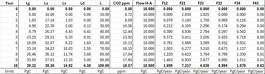
Here is table “Berry Carbon Flow Test” for discussion in our comments.
I request Ferdinand and anyone else who is contesting my calcuations to present your calculations for comparison.
We assume that the natural carbon cycle is at constant levels as shown in Figure 3.
With that information, we insert human carbon into the atmosphere at a constant rate of 10 PgC per year. Then we calculate annual time steps to see how much human carbon ends up in each reservoir each year.
This simple calculation is a way to compare our calculations because we keep human carbon inflow constant for each year.
The years run from zero to ten. All the L data are in PgC, and flow data are in PgC/Year.
Lg = land, La = atmosphere, Ls = surface ocean, Ld = deep ocean, L is the total PgC in the carbon cycle for each year. Ntice L increases by 10 PgC each year.
The CO2 ppm column simply converts the PgC in La to ppm.
Here’s how it works.
Year 0: 10 PgC is added to La, but you don’t see it until the beginning of Year 1.
Year 1: the 10 PgC in La produces outflows to Lg and Ls. We see the result in Year 2.
Year 2: the outflows from La have moved some carbon to Lg and Ls. Etc.
Notice that as La gets more PgC, its Outflow to Lg and Ls increase, etc.
While La increased by 7.14 PgC from Year 1 to Year 2, it increased by only 1.49 PgC from Year 9 to Year 10.
Also notice that as Lg and Ls get more carbon, they send carbon back to La.
Adjustment, Residence, E-time Compared
IPCC’s response times fail physics
Physics e-time has a precise definition. The IPCC times do not. In summary:
- Physics: e-time is the time for the level to move (1 – 1/e) of the distance to its balance level.
- IPCC: adjustment time is the time for the level to “substantially recover” from a perturbation.
- IPCC: residence time is the average time a CO2 molecule stays in the atmosphere.
IPCC defines “adjustment time (Ta)” as:
The time-scale characterising the decay of an instantaneous pulse input into the reservoir.
Cawley defines “adjustment time (Ta)” as:
The time taken for the atmospheric CO2 concentration to substantially recover towards its original concentration following a perturbation.
The word “substantially” is imprecise.
Cawley follows IPCC to define “residence time (Tr)” as:
The average length of time a molecule of CO2 remains in the atmosphere before being taken up by the oceans or terrestrial biosphere.
In summary, IPCC uses two different response times where it should use only e-time:
- When the level is far from its balance level (which can be zero), IPCC thinks e-time is an adjustment time because the level is moving rapidly toward its balance level.
- When the level is close to its balance level, IPCC thinks e-time is a residence time because “molecules” are flowing in and out with little change in level.
Figure A illustrates how e-time relates to IPCC’s adjustment and residence times.
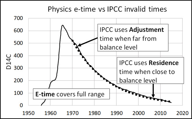
Figure A. E-time covers the full range of movement of level to a balance level. IPCC adjustment and residence times apply to only each end of the range.
IPCC, 2001: Working Group 1: The scientific basis. Appendix 1 – Glossary.
Lifetime
Lifetime is a general term used for various time-scales characterising the rate of processes affecting the concentration of trace gases. The following lifetimes may be distinguished:
Turnover time (T) is the ratio of the mass M of a reservoir (e.g., a gaseous compound in the atmosphere) and the total rate of removal S from the reservoir: T = M/S. For each removal process separate turnover times can be defined.
Adjustment time or response time (Ta) is the time-scale characterising the decay of an instantaneous pulse input into the reservoir. The term adjustment time is also used to characterise the adjustment of the mass of a reservoir following a step change in the source strength.
Half-life or decay constant is used to quantify a first-order exponential decay process.
The term lifetime is sometimes used, for simplicity, as a surrogate for adjustment time.
In simple cases, where the global removal of the compound is directly proportional to the total mass of the reservoir, the adjustment time equals the turnover time: T = Ta.
In more complicated cases, where several reservoirs are involved or where the removal is not proportional to the total mass, the equality T = Ta no longer holds.
→Carbon dioxide (CO2) is an extreme example. Its turnover time is only about 4 years because of the rapid exchange between atmosphere and the ocean and terrestrial biota.
However, a large part of that CO2 is returned to the atmosphere within a few years.
Thus, the adjustment time of CO2 in the atmosphere is actually determined by the rate of removal of carbon from the surface layer of the oceans into its deeper layers.
Although an approximate value of 100 years may be given for the adjustment time of CO2 in the atmosphere, the actual adjustment is faster initially and slower later on.
From Ferdinand Engelbeen, July 10, 2025 at 1:41 pm and Jim Siverly, July 10, 2025 at 4:41 pm
This may be a bit premature, but if I don’t write it now, it may be gone forever.
From Ferdinand’s power point presentation at a Clintel wrokshop in Athens, last September (see his comment on July 10, 2025 at 3:43 am), I saw Tau defined as the usual disturbance / effect. However, there was a slide with the example:
Tau = (415 uatm – 295 uatm) / 2.35 uatm/year = 51 years
I interpret the denominator as the difference between the current CO2 level and what it was in preindustrial times. The numerator is the current CO2 sink rate. While I am still waiting for a formal presentation of the derivation of that equation, I was curious what would happen to my spreadsheet model if I ran it from 2018 (the last year of my available industrial emission data) until equilibrium assuming no further industrial emissions and a freeze of the natural emissions at the 2018 level. My model uses a 4-year residence time (turnover, e-time, etc.) and allows for an exponentially increasing biomass. In other words, the land and ocean reservoirs average more emissions gradually each year from 65 ppmv to 93 ppmv. The increase was necessary to correlate with the Mauna Loa data.
The model simulation resulted in an equilibrium value of 398 ppmv in 2045, down from 410 ppmv in 2018. The 1/e value of about 402 ppmv occurred in 2022 or about four years.
My hypothesis is this: no matter what the equilibrium CO2 level would be, if the world suddenly went net zero, the new CO2 would be at that new level in less than 30 years with a 63% reduction in only four years.
Re: Uncle Bert’s comment July 10, 2025 at 10:13 am
Dear Uncle Bert.
More excuses and specious waffle and totally lacking in any science. The deeper you dig yourself into the quagmire the more difficult it is to make any sense out of anything that you say. Everything you write is specious. Unvalidated assumptions and pseudoscientific rhetoric. I find myself agreeing with Jim Silverly. Your ideas are an artifact of your self-fulfilling prophecy. “the compilation of the late Ernst Beck makes no sense”. Any measurement that doesn’t fulfill your self-fulfilling prophecy makes no sense to you.
200,000 measurements from 901 locations from dozens of highly qualified and notable scientists produce data that doesn’t conform to the confirmation bias of the catastrophic anthropogenic global warming CAGW proponents so they invented a new term. “Background layer”. CO2 is well mixed everywhere unless it’s near one of the accurate scientific instruments from the 1812 to 1961 instrumental record. So the CAGW proponents invented a fictitious “background layer” just to cloud the argument.
“The standard deviation for the historical CO2 data was 68 ppmv (1 sigma, not a sign of reliability!), of the modern station about half of it”
You’re comparing monotonic ice core proxy data to Mauna Loa measurements. All that does is demonstrate you’re not a scientist and have no scientific argument.
“And the ice core from the Siple core (not the Byrd core) indeed was contaminated with drilling fluid”
Jaworowski produced measurements that doesn’t conform to your confirmation bias so you have to invent something wrong with it and attack the man. You fail to admit that all ice cores have drilling fluid contamination. Jaworowski’s had less than ALL the others and probably none at all.
Then the 1812 to 1961 instrumental measurements were not what you wanted so you’ve concocted a specious argument that they were contaminated from all the fly and insect farts. They only thing that’s contaminated is your brain.
“a simple calculation, based on observations, is as valid as a direct observation”
Calculations that give you the confirmation biased results that you are looking for are not measurements. You take real measurements, put them through a calculation and produce fake results.
Uncle Bert. You need to retire to your IPCC cubicle and retire from bring a political agitator. Do something meaningful with your life. Get a life.
I don’t know about the rest of you but I have lost my patience trying to wade through all of Uncle Bert’s specious waffle. It’s endless. It’s like how the Indians say they are drunk. Translated – “my head is eating circles”. As fast as the specious waffle comes around, you chew it up and spit it out but it just keeps coming around and around. They say when you die and go to Heaven, that’s if we all make it there, that life is eternal. I think there’s something after that for Uncle Bert’s specious waffle.
David Andrews
July 10, 2025 at 8:13 pm
David,
The “fossil only” issue arose in my comment (July 10, 2025 at 10:10 am) following Dave Burton’s at July 9, 2025 at 4:35 pm. I said, “You even label the graph “fossil only” seemingly unaware of the fact that it violates the equivalence principle.” Dave explained that “fossil only” meant omitting the land use fraction of industrial carbon. Got that so far?
OK, then I went back to look at the plot equation which is based on Eh(t) – dC(t)/dt = Sn(t) – En(t). The left-hand side basically means “fossil carbon not removed” in year t. It violates the equivalence principle, because the full Eh(t) that year is mixed in with the rest of the atmosphere and much more than half of Eh(t) gets removed.
Am I missing what you mean by carbon conservation? If you mean simple math as in the equation above, then we have a problem. And I think it’s because we don’t share the same understanding of the equivalence principle.
Jim Siverly July 10, 2025 at 9:58 pm
“My model uses a 4-year residence time (turnover, e-time, etc.) and allows for an exponentially increasing biomass. In other words, the land and ocean reservoirs average more emissions gradually each year from 65 ppmv to 93 ppmv. The increase was necessary to correlate with the Mauna Loa data.”
The basic problem is that one can match the Mauna Loa data with any combination of (net) sinks and temperature…
Thus one need to look at the physics behind the math.
The 4 years residence time of today includes all inflows and outflows, whatever their direction. Including two main cycles: from the warming oceans through the atmosphere to increasing vegetation in spring/summer and back in fall/winter. These cycles are near completely independent of the actual CO2 pressure in the atmosphere.
Indeed they did increase over (many) years, as you assume, but from the past to today that is only true in ratio for the ocean surface (according to the IPCC, but they didn’t give any explanation how and why that happens) and less than complete for the biological cycle: some 40% increase in the cycle for the CO2 increase in the atmosphere, despite 175 years time to get the same percentage.
Your thesis implies that the current equilibrium increased at about the same rate as the increase in the atmosphere, matching the 4 years residence time to allow for the difference.
A new equilibrium will be approached with a Te of 4 years at about 398 ppmv in 2045.
So far so good. Only one problem: the 398 ppmv is way above the equilibrium pCO2 of the oceans surface, which would be around 295 μatm (~ppmv, ppmv is in dry atmosphere, μatm in the atmosphere includes water vapor).
If we simply ignore the ice core results and start in 1958, the level in the atmosphere was 315 ppmv.
Assuming an equilibrium pCO2 of the oceans, that also starts at about 315 μatm in 1958.
With the increase in temperature, the pCO2 of the ocean surface increases with the formula of Takahashi:
(pCO2)seawater @ Tnew = (pCO2)seawater @ Told x EXP[0.0423 x (Tnew – Told)]
or with an increase of 0.6°C (HadSST3 global) that increases the overall pCO2 of the sea surface waters to:
pCO2(new) = 315*EXP(0.0423*0.6) = 323 μatm.
Less than 10 μatm increase in equilibrium pCO2 by the ocean surface over the period 1958-2025.
Vegetation hardly plays a role in the equilibrium: they watch and wane with the overall pCO2 in the atmosphere, which is determined by the ocean surface waters over the millennia and the availability of land in between ice ages.
That can be seen in the very small changes in δ13C over the past 800,000 years, despite huge changes of 90 ppmv in CO2 level, until humans started to emit FF CO2:
https://www.ferdinand-engelbeen.be/klimaat/klim_img/co2_d13C_lgm_cur.png
Even with an enormous increase in size between glacial and interglacial periods: that is completely dwarfed by the equilibrium set by the ocean surface temperature and the changes in size were slow enough to get equalized by the deep oceans cycle.
Moreover, if you calculate the equilibrium pCO2 down to where inflows and outflows are equal (thus zero net flow), over the period 1958-current, that shows a level of 285 ppmv. Here from David Burton:
https://sealevel.info/Global_Carbon_Budget_2023v1.1_with_removal_rate_plot2.png
That is only calculated from the observed net sink rates, thus independent of any idea of the real level of Te or Tau.
Again the “old” equilibrium that didn’t change much over time.
For the underlying equations of the long Tau of around 50 years: already obtained in 1997 by Dipl.-Ing. Peter Dietze in a debate with the inventor of the Bern model, Fortunat Joos:
https://www.ferdinand-engelbeen.be/klimaat/klim_img/Dietze_1997.png
More on that page at the website of the late John Daly:
https://www.john-daly.com/carbon.htm
And the discussion with Joos and others:
http://www.john-daly.com/dietze/cmodcalc.htm
https://www.john-daly.com/dietze/cmodcalD.htm
Jim Siverly, July 10, 2025 at 10:39 pm
Eh(t) – dC(t)/dt = Sn(t) – En(t)
Eh(t) is the human input, for 100% injected into the atmosphere as mass.
That increases the total mass of CO2 in the atmosphere.
– dC(t)/dt removes a certain amount of mass of CO2 out of the atmosphere, no matter the composition, thus original human and natural CO2 molecules alike, and that equals natural sinks minus natural sources, because of a lack of human sinks (again as mass, not in original FF molecules)…
Everybody of the “man-made” CO2 increase is talking about carbon mass transfers, only the “natural-made” CO2 increase people make a differentiation…
Jim Siverly July 10, 2025 at 4:41 pm
Unfortunately, the Wiki page had their simple formula of the decay rate for a linear ratio process on the same page as today for the exponential decay rate, but someone deleted it.
Anyway Peter Dietze in 1997 and many others after him (Lindzen, Spencer) used the same formula to calculate the effective adjustment (or life) time.
If there is a linear ratio between cause and effect, it doesn’t matter over what time frame Tau is calculated. In the case of the recent record since 1958, one can calculate Tau over 1 year (as I have done, be it on the smoothed sink rate) or over a period of 10 years or over the full period, you will obtain the same result. Of course, by using the polynomial, the results are already smoothed…
The sentence:
“Effect in the case of CO2 is the net increase in output when the CO2 level above the equilibrium increases, the net increase in output is the difference between inputs and outputs, for each bidirectional exchange between reservoirs apart as good as for all exchanges together.”
means that one can calculate the different Tau’s for each exchange between the atmosphere and the different reservoirs, if one knows the net outflux (that is difference between inputs and outputs) for each of them.
In that case total Tau(c) can be expressed as function of n exchanges:
1/Tau(c) = 1/Tau(1) + 1/Tau(2) +… …+ 1/Tau(n)
Dr. Ed, July 10, 2025 at 7:19 pm
Dear Dr. Ed,
Only one remark:
“Total human carbon has added one percent to the carbon in the natural carbon cycle”
I think that we all agree that human emissions get into the atmosphere for the full 100%, thus adding some 10 PgC/year to a total of CO2 that circulates through the atmosphere with 200 PgC/year as input and 205 PgC/year as output for the current CO2 cycles.
For the mass balance, the human input is the first cause for the increase of 5 PgC in the atmosphere, or you violate the mass balance. That is about mass transfer.
For the molecular balance, if the FF CO2 is only 1% of all CO2 in the atmosphere and nothing comes back with the return flows, the removal of FF molecules is 2.05 PgC/year, still near 8 PgC/year of FF molecules are added to the atmosphere each year.
Further, as the 2 PgC/year FF molecules are distributed into ocean surface and vegetation via the fast cycles, some of these FF molecules will return from the other reservoirs, increasing the FF molecular level in the atmosphere.
On the other hand, the increase in FF molecules also increases its ratio in the outputs…
The current, measured, increase of FF molecules in the atmosphere is already over 10% and in the ocean surface over 6%. In vegetation and deep oceans also increasing, but difficult to quantify. The former does only return waters with CO2 from ~1000 years ago, that does influence the current 13C/12C and Δ14C levels.
In short: The full input of FF CO2 gets into the atmosphere and gives its full increase in the atmosphere as mass and an enormous drop in 13C/12C ratio. About half that input as mass (whatever the origin) is removed and about 2/3 of that input as original FF molecules is replaced by CO2 molecules from other reservoirs…
Brendan Godwin, July 10, 2025 at 10:22 pm
A last comment to your “science”, as I see that it is just a waste of my time to discuss things with someone who doesn’t want to accept any data which he doesn’t like.
– “200,000 measurements from 901 places”
Of which 198.000 contaminated with local sources and sinks. Completely worthless to know the past global CO2 levels.
Those measurements that were over sea and coastal with wind from the seaside are on or below the ice core measurements. On or below. No peak at all in all the measurements over the oceans. Strange isn’t it?
https://www.ferdinand-engelbeen.be/klimaat/klim_img/beck_1930_1950.jpg
The minima are, not by coincidence, mostly from measurements over the oceans or coastal
That is already 70% of the global surface.
Then we have recent flight measurements, here over the Rocky Mountains:
https://www.ferdinand-engelbeen.be/klimaat/klim_img/inversion_co2.jpg
Once over 700 meters, the CO2 levels are within a few ppmv of the Mauna Loa level for the same days.
In total: 95% of the air mass shows “background” CO2 levels within 10 ppmv from near the North Pole (Barrow) to the South Pole.
But according to Brendan, we should believe the historical (and current?) CO2 measurements in 5% of the atmosphere from highly contaminated areas over land.
– “You’re comparing monotonic ice core proxy data to Mauna Loa measurements. All that does is demonstrate you’re not a scientist and have no scientific argument.”
The ice core data are direct measurements of CO2 in the atmosphere, not “proxies”. Including an overlap of 20 years with the direct measurements at the South Pole. If you have any real “scientific” arguments, why we shouldn’t use these data for historical CO2 levels, then give them…
And I was comparing the historical CO2 data from Giessen:
https://www.ferdinand-engelbeen.be/klimaat/klim_img/kreutz_08.jpg
Which show a range of 240-680 ppmv (wow, what a “background” range – CO2 at that time was expressed as tenths of a percent) and a standard deviation (“streuung”) of 66 ppmv with the
stdev of the modern station at Linden/Giessen of around 30 ppmv
and with the Mauna Loa stdev of some 2 ppmv and
the South Pole data stdev of less than 1 ppmv
and the ice cores with a stdev of 1.2 ppmv
If you have any scientific arguments why we should use the historical data from Giessen as the “real” background CO2 level of that time, be my guest.
– Jaworowski produced measurements that doesn’t conform to your confirmation bias
Jaworowski never, ever did any CO2 measurement in ice cores. He did measurements in ice fields of Scandinavia for the radioactive fallout of the Tsjernobyl disaster.
These icefields are at much higher temperatures than the Greenland or Antarctic ice cores and therefore have a lot of water veins where metal ions can migrate. That is near impossible for CO2 in ice cores at -20°C to -40°C.
Thus his critiques were based on quite different materials and circumstances.
One has calculated the theoretical migration of CO2 in the Siple Dome ice core by looking at the increase of CO2 near a melt layer. The conclusion: at middle depth the resolution increases with some 10% or from about 20 years to 22 years and near the bottom rock it doubles from 20 to 40 years. And near melt layers, on can find higher than average CO2 levels. Melt layers are typical for the Siple Dome ice core and absent in Law Dome and, as far as I know, any other Antarctic ice core.
Simply not important at all for migration and not measurable in any ice core that is colder:
https://catalogue.nla.gov.au/catalog/3773250
Bye bye…
Stephen P. Anderson, July 10, 2025 at 3:12 pm
“The partial pressure of CO2 is equal to the mole fraction of CO2 times the total pressure of the atmosphere. It has nothing to do with some imaginative pCO2(ocean).”
Of course the pCO2 is what you describe, but you are wrong about the pCO2 of the oceans: That is the base for Henry’s law and describes the partial pressure of the oceans in equilibrium with a small volume of air above it. That pCO2 is measured in the small air volume and is used as pCO2 of the ocean water.
When the pCO2 of the oceans and the atmosphere above it are equal, there is no net CO2 transfer between the two (still a lot of CO2 molecules are traveling in each direction, but flows are equal up and down).
The pCO2 of the oceans was measured with meanwhile several millions of samples, even on commercial sea ships with automatic equipment on board…
See further the compilation of Feely et al. for the reference year 1995:
https://www.pmel.noaa.gov/pubs/outstand/feel2331/maps.shtml
for the overall formula to calculate the net CO2 flux between atmosphere and oceans, based on the difference in pCO2 between atmosphere and ocean surface waters.
The whole interesting story starts about at:
http://www.pmel.noaa.gov/pubs/outstand/feel2331/exchange.shtml
Jim (and Ed too),
Ferdinand has responded to Jim’s equivalence principle concern, but I will too. Let’s go back to the beginning.
(change rate of atmospheric carbon) = (carbon addition rate by all processes) – (carbon removal rate by all processes).
Divide the PROCESSES into human and natural and indicate which by subscripts. MAKE NO DISTINCTIONS ABOUT CARBON TYPES OR YOU MAY GET CONFUSED.
Processes which add are E(missions). Processes which remove are A(bsorptions)
dC/dt = En + Eh – An – Ah
En = ocean outgassing, vegetation decay, etc
Eh = human burning of fossil fuels
An = dissolution of carbon into the oceans, photosynthesis, etc
Ah = removal by direct carbon capture technology, sequestration, etc. Unless you can name a human PROCESS which removes carbon of any type on the scale of Petagrams, we will ignore this term.
Then Eh-dC/dt = An – En
It is usually easiest to integrate this over time, and talk about stock changes in a fixed period.
The left-hand side is definitively measured to be positive in the industrial era. Therefore, the right-hand side is too. Natural processes are definitively removing more carbon from the atmosphere than they are adding.
Good luck making a model which says the human influence is small.
David Andrews July 11, 2025 at 9:48 am
Dear David,
Let’s use your equation:
dC/dt = En + Eh – An – Ah ………………(1)
Argument #1
Equation (1) works for natural and human processes individually:
dCn/dt = En – An…………………….(2)
dCh/dt = Eh – Ah…………………….(3)
Assume (2) is at equilibrium, so it is zero. Then we can easily find the six Te from IPCC’s data for its natural carbon cycle at equilibrium.
Then we can integrate (3) from 1750 to 2020 using data for annual human CO2 emissions.
By using the same Te in (3) as found in (2), we can calculate how fast human CO2 flows out of the atmosphere annually.
This is the key.
Human CO2 will flow out of the atmosphere and into the other carbon reservoirs, in proportion to its level, exactly as fast as natural CO2 is already flowing out of the atmosphere.
Human CO2 is a minor part of the total CO2 flows, so it can’t change the rules, or Te.
The sum of (3) from 1750 to 2020 is much less than the measured total CO2 increase.
This means your argument is wrong because you ignored the annual outflow of human CO2.
Therefore, nature did not stay at equilibrium from 1750 to 2020. Nature played a dominant part in the CO2 increase.
Argument #2
Rewrite (1) as follows:
dC/dt = (En– An) + (Eh – Ah) ………………………………. (4)
Integrate (4) from 1750 to 2020 to get:
Total CO2 increase = (Natural CO2 increase) + (Human CO2 increase)………………….(5)
This shows your argument depends on what you assume for Natural CO2 increase.
If you assume the natural increase is zero then you automatically conclude all the increase was Human CO2 increase.
When you drop Ah, you are assuming all the increase was Human CO2 increase. Therefore, your reasoning is circular, and wrong.
Ferdinand Engelbeen July 11, 2025 at 7:59 am
Dear Ferdinand,
Neither of your referenced articles negate my formulation that uses (1) and (2).
The proper use of such information is to fine tune my formulation.
But the proper way to fine tune my formulation might be to begin by expanding the number of land reservoirs and ocean reservoirs. That would allow simulation of different types of land and allow consideration of ocean flow.
The key to doing this is my formulation because it easily allows such expansion to multiple reservoirs and addition of flows between the new reservoirs.
As everyone knows, no model can perfectly describe nature. But my model comes closer than any other model because it is based on only two equations.
Ferdinand Engelbeen July 11, 2025 at 4:36 am AND July 11, 2025 at 7:59 am
Dear Ferdinand,
Please see my reply to David Andrews July 11, 2025 at 9:48 am
All arguments about the carbon cycle or “carbon mass balance” must use equations and numbers. Your use of numbers is not a valid argument because you are not showing where your numbers enter equations.
That’s why we must first agree on the formulation of the problem. Until then, numbers such as you and Dave Burton throw out have no relevance to our discussion.
I have provided the only complete formulation of the problem, and I have provided the way to numerically integrate levels and flows over time.
Until someone does a competing formulation, my formulation is the only game in town.
Ed,
You persist in being willfully ignorant by, once again, conflating human/natural processes with your “human/natural carbon”, despite my BOLD CAPS WARNING that doing so would confuse you. I made the “mass-balance” argument as clear as I could, but evidently it was not clear enough for “Winterberg’s best student”. I hope it was clear enough for Jim, but I am not optimistic. His logic has been kind of shakey recently.
Congratulations, once again. You have confirmed Hans Seuss’s 1955 comments about what are now called disequilibrium isofluxes. Indeed, your “human carbon” is but a small part of the present atmosphere as he predicted. But that is irrelevant to determining the cause of the CO2 increase. The mass-balance argument tells us about that. You have not refuted it. Obviously I have nowhere assumed anything about the constancy of natural processes. Data show clearly that natural sinks are increasing in response to the higher carbon levels in the atmosphere.
Ed, David, and Ferdinand,
Not that you are waiting with bated breath, but I am anxious to respond, busy until later today, and will respond sometime, hopefully.
Dr. Ed,
David Andrews has said it very correct.
But let’s go in more detail again. The whole discussion is about what caused the increase in CO2 mass in the atmosphere. Not where the human FF molecules reside or are transferred to. Even if they are all captured by the next available tree within seconds, that excludes the capturing of a natural CO2 molecule in the same season, except for a small increase in biomass over a year.
dC/dt = En + Eh – An – Ah
Where dC/dt and Eh are quite exactly known and Ah as human induced sink of CO2 mass (not sinks of human FF molecules!) is negligible.
Thus even if we don’t know En and An exactly, and thus the margins of the residence time Te are rather wide, we do know the difference between En and An quite accurately.
For the past years we can make the rough sums (as mass) in PgC/year:
dC/dt = 200 (En) + 10 (Eh) – 205 (An) – 0 (Ah)
Both En and An do already contain a certain percentage of FF molecules, but that is about transfer of molecules, and only of academical interest, as that doesn’t have any influence on the measured transfer of CO2/carbon mass, whatever its composition.
What is sure, is that all FF emissions as mass and as isotopic composition are for 100% injected into the atmosphere.
With 909 PgC in the atmosphere (2025) we have, with Te(c), the overall residence time of CO2 in the atmosphere:
Te(c) = 909 / 205 = 4.43 years
With a difference of CO2 in the atmosphere between 2025 and 1750 we have:
Tau = (909 – 589) / (210 – 205) = 64 years
A little overblown as the zero net outflow equilibrium slightly increased from 1750 to 2025 due to warming oceans from 589 PgC to 628 PgC which gives:
Tau = (909 – 628) / 210 – 205) = 56 years
So, which one is of interest?
Te is based on the sum of all outputs out of the atmosphere, no matter their direction or back flows from the receiving reservoir. Even if the back flows from oceans and vegetation were equal to the outflows from the atmosphere into the oceans and vegetation, Te will not change. But the net CO2 transfer from the atmosphere to the two main other reservoirs would be zero.
As the exact flows between the different reservoirs are only known with large margins of error and the flows between ocean surface and deep oceans not measured at all (that is based on the Bern model!), any calculation of the net outflow based on the residence times is very problematic.
The only time of interest is Tau, which shows how much net CO2 really get transferred from the atmosphere into the other reservoirs. The only point of discussion in that case is the shift of the equilibrium over time since 1750, but that is easily solved by using the formula of Takahashi for the increase of pCO2 of the ocean surface with temperature, confirmed by the back calculation of the measured net CO2 output to zero net output by David Burton and many others in the past:
https://sealevel.info/Global_Carbon_Budget_2023v1.1_with_removal_rate_plot2.png
DAVID ANDREWS JULY 11, 2025 AT 8:57 PM
Dear David,
My simple demonstration using your own equation proves your interpretation of your equation is wrong.
You responded, as you always do when trapped, by attacking me personally, which is a giveaway that you are wrong.
You wrote:
Irrelevant?
Then show it in math, David. Show it in math.
Your capitalized statement is scientific insanity:
Wow! In theoretical physics, David, we always explore the next level of detail to get as much information as we can. And in this debate, that obvious next level is to consider human and natural carbon independently.
After all, the objective of this debate is to determine the effects of human CO2 emissions, as distinct from natural CO2 emissions. We can’t do that unless we look at each process separately.
We lose no information is this logical separation but we gain more insight. And that separate insight proves you are wrong.
That’s how we do theoretical physics, David. But you never learn.
You refuse to look at each process separately because you realize you lose the debate when we do.
(Yes, I was Winterberg’s best student, by far, as he wrote several times. Care to compare your PhD thesis with mine? My bet is you cannot follow the math and logic in my thesis, which was a breakthrough in climate physics, described in textbooks, exclaimed by Russian physicists, and still gets several citations every year. And, yes, I did score a perfect 800 on my SAT and finished in half the allotted time because the test should have been twice as long.)
Dr. Ed, July 11, 2025 at 12:18 pm
“When you drop Ah, you are assuming all the increase was Human CO2 increase. Therefore, your reasoning is circular, and wrong.”
We didn’t “drop” Ah for circular reasoning, Ah just is minuscule and less than 1% of Eh…
Your calculations should show:
F(a-g) – F(g-a) + F(a-s) – F(s-a) + F(s-d) – F(d-s) = dC/dt – Eh
As you use the overall Te of around 4 years in your calculation, the result is far too small and doesn’t reflect the real increase in the atmosphere.
Again, somewhere lost in the discussion:
With your Te of 4 years, most human emissions are redistributed into vegetation and oceans.
Despite that, there is a measured increase of CO2 in the atmosphere.
What is then the source of that extra CO2, as both oceans and vegetation increased in carbon content?
Ed,
“That’s why we must first agree on the formulation of the problem.”
Yes, we must agree on the formulation of the problem. I think we agree that the problem is to determine: “what has caused the atmospheric CO2 increase over the last century?”
Your formulation is to calculate the “human carbon” in the present atmosphere. Your central conceptual error is to not recognize, or at least not acknowledge, that this is an unimportant statistic determined by the mixing, on a short residence time scale, of atmospheric carbon with that in other reservoirs. Balanced mixing does not change levels, as illustrated by my little thought experiment. I know you care deeply about this unimportant statistic because it is your signature contribution, praised by coal man Richard Courtney. But your separate tracking of human and natural carbon has gotten you nowhere useful. It is the total carbon that matters, and that is tracked by the mass-balance analysis.
Between 1960 and 2010
350 +- 29 PgC of human emissions
158 +- 2 PgC of atmospheric accumulation
Therefore 192 +- 29PgC of net global uptake, because the carbon we added has to be accounted for.
The argument is remarkably simple and makes no assumptions about the constancy of natural processes. If you can discipline yourself not to go off on unnecessary tangents about different carbon types, you will see it too.
Ferdinand Engelbeen July 12, 2025 at 7:10 am
Dear Ferdinand,
Thank you again for your participation in this debate.
As you say, “The whole discussion is about what caused the increase in CO2.”
For this discussion, I have the option to rewrite our (1) as my (4)
dC/dt = (En– An) + (Eh – Ah) ………………………………. (4)
which when integrated over a period of years becomes:
Total CO2 increase = Total (En– An) + Total (Eh – Ah)………….(6)
Which is the same as my (5).
Now, we can insert your “rough sums” to get (6):
Total CO2 increase = Total Natural (200 – 205) + Total Human (10 – 0)………….(6a)
Hmm. It looks like your rough sums say the following:
Total CO2 increase = Total Natural (-5) + Total Human (+10)………….….(6b)
Your rough numbers say nature subtracted 5 and human added 10.
Do you really believe that? I don’t. But those are your numbers.
Further, I don’t agree at all with your definitions and calculations of Te and Tau. We can discuss these disagreements after you fix your numbers to make (6b) believable.
David Andrews July 12, 2025 at 11:15 am
Dear David,
Your physics is clutzy. Please put your numbers into equation (6) that I just wrote in my comment to Ferdinand:
Total CO2 increase = Total (En– An) + Total (Eh – Ah)………….(6)
Using Ferdinand’s numbers, this became:
Total CO2 increase = Total Natural (200 – 205) + Total Human (10 – 0)………….(6a)
Total CO2 increase = Total Natural (-5) + Total Human (+10)………….….(6b)
Ferdinand Engelbeen July 12, 2025 at 10:53 am
Dear Ferdinand,
Your following equation does not properly represent my calculations:
F(a-g) – F(g-a) + F(a-s) – F(s-a) + F(s-d) – F(d-s) = dC/dt – Eh
However, we have a bigger problem.
You claim Ah is less than 1% of Eh.
Your conclusion is based on your other errors. We must begin with IPCC’s natural carbon cycle data, shown in my Figure 3.
Then you have some problems to solve:
1. Your Tau of 50 years does not fit IPCC’s natural carbon cycle data.
2. Your Tau of 50 years does not fit the bomb test data that show Te = 16.5 years with a balance level of zero.
3. Your Tau is the time for a level to move 63% of the way to its balance level. Well, that is exactly Te. So, you have no basis to claim a Tau of 50 years, which is the same as saying Te is 50 years.
4. You assume human CO2 moves out of the atmosphere with a Tau of 50 years and then you conclude from this assumption that “Ah is less than 1% of Eh.”
5. You have not made a valid argument to justify your conclusion. Even IF you think Ah is small that does not justify dropping it from your equation.
6. Salby and Harde found that CO2 flows out of the atmosphere with Te much less than 3.5 years. You can see this in the monthly CO2 data. If your Tau of 50 years were in control, there would be no monthly sawtooth pattern in the CO2 data.
7. Your claim that H(1) is true conflicts with Munshi’s statistical analysis that shows the annual correlation of human CO2 emissions with annual CO2 increase is zero, which proves H(1) is false.
Dr. Ed, July 12, 2025 at 11:27 am
“Total CO2 increase = Total Natural (200 – 205) + Total Human (10 – 0)………….(6a)
Hmm. It looks like your rough sums say the following:
Total CO2 increase = Total Natural (-5) + Total Human (+10)………….….(6b)
Your rough numbers say nature subtracted 5 and human added 10.”
Indeed that is exactly what David and David and I are saying…
There simply is no appreciable human sink in this entire world… The only sinks are natural sinks, which absorb any mix of natural and human CO2 alike.
Even if you integrate all human emissions in the period 1958-2020, that is about 170 ppmv, while the measured increase is only 100 ppmv. Nature removed 70 ppmv CO2 out of the atmosphere into oceans and vegetation…
https://www.ferdinand-engelbeen.be/klimaat/klim_img/acc_co2_mlo_t_1960-cur.png
Ferdinand Engelbeen July 12, 2025 at 12:41 pm
Dear Ferdinand,
You say,
“Indeed, that is exactly what David and David and I are saying…
There simply is no appreciable human sink in this entire world… The only sinks are natural sinks, which absorb any mix of natural and human CO2 alike.”
That statement sinks your ship.
Even as you admit there are natural sinks, you are saying that there are no human sinks.
Does that begin with the first human CO2 molecule? Or the first ten?
You are saying that the jillions of trees on the planet will not accept the CO2 added by human emissions. This contradicts even the famous picture of four trees grown in different CO2 levels.
So, you are saying that the Te for human CO2 is much greater than the Te for natural CO2. Your argument violates the climate equivalence principle.
With this, I am outa here. Got better things to do today.
Ed,
I hadn’t seen your 10:38 post when I wrote my 11:15 post. Now I see your 11:47 post and later ones too.
A few points:
1. For a semi-quantitative analysis of why your calculation of “human carbon” in the present atmosphere is irrelevant, see my rebuttal to Skrable. https://pubmed.ncbi.nlm.nih.gov/36719939/ The mixing means that only about the last decade’s worth of C14 devoid “human carbon” should be expected to still remain in the atmosphere. That agrees well with the current measured atmospheric radiocarbon specific activity. This is the diluted Seuss effect which you have shown you are uncertain about even though you effectively calculated it. No one ever expected to measure the (undiluted) “Natural + 33% Human” curve in your Figure 9, because the composition of the present atmosphere only gives information about the last decade; earlier information is effectively erased by the mixing. I could make the case that my argument on the Skable analysis shows that, in the last decade at least, the rise is anthropogenic. Similarly the pre-1950 data shows a (diluted) Seuss effect. But a conservative conclusion is just to say that the present atmospheric composition is an unreliable indicator by itself of the atmosphere’s history because of mixing. Interpreting the composition as showing that the CO2 increase is mostly natural as you do, as if mixing doesn’t occur, is naïve and just plain wrong.
2. You make a case for analyzing details in physics, such as studying the human and natural cycle separately. Yes, that is often the case. I think the reason you are the only one doing it here is to be found in the paragraph above. And I am sure you know of many, many physics problems where the smart approach is to apply a conservation law rather than to grind through an unnecessarily detailed analysis. Carbon conservation is a quite useful constraint.
3. On your request that I insert numbers into your (6) to attribute the atmospheric growth to natural or human origins: I will use the Ballantyne numbers again, for the period 1960-2010, omitting error bars this time. The units are PgC
Total Increase = 158
Human input = 350
Natural input = -192
Yes, things would be a lot worse if natural sinks weren’t bailing us out. The ~45% “airborne fraction” has held up pretty well.
4. I see you are still haggling with Ferdinand about “Ah”. He is correct. Did you bother to read how I defined it?
Dr. Ed, July 12, 2025 at 12:37 pm
Dear Ed,
“Your following equation does not properly represent my calculations:
F(a-g) – F(g-a) + F(a-s) – F(s-a) + F(s-d) – F(d-s) = dC/dt – Eh”
Indeed, it shows what your calculations should show, but don’t show…
dC/dt and Eh both are quite exactly known. dC/dt – Eh is the overall removal of CO2 wherever in nature that may be, for human and natural CO2 together, whatever the mix in the atmosphere.
All bidirectional fluxes between the atmosphere and vegetation or oceans together should equal the net sink rate of what is removed out of the atmosphere as mass.
Then the other items:
“You claim Ah is less than 1% of Eh.”
Again… Ah is what humans exactly produce as CO2 mass sinks. That are things like reforestation in some countries, still dwarfed by clear cutting of forests in other countries, CCS (pretty good object for government subsidies, but the largest project did fail), etc. That is not about how much original FF molecules are removed with the increasing outflows into oceans and vegetation.
“1. Your Tau of 50 years does not fit IPCC’s natural carbon cycle data.”
The Tau of 50 years is calculated from the difference between the current CO2 level in the atmosphere with the “old” equilibrium (plus T influence) and the observed net outflow. Tau has nothing to do with CO2 cycles.
“2. Your Tau of 50 years does not fit the bomb test data that show Te = 16.5 years with a balance level of zero.”
The Te of 4 years also doesn’t fit, but you forget the “thinning” of the δ13C and Δ14C signals by the deep ocean returns of ~1000 years ago with 13C/12C and Δ14C of long before the bomb tests and fossil fuel use.
And you forget the 14C-free supply of FF…
That makes that the decay rate for Δ14C is much faster than for 12/13CO2 as mass and that the drop of δ13C is only 1/3 of what it should be if all FF remained in the atmosphere…
“3. Your Tau is the time for a level to move 63% of the way to its balance level. Well, that is exactly Te. So, you have no basis to claim a Tau of 50 years, which is the same as saying Te is 50 years. ”
You did calculate a Te of 4 years by adding all outputs out of the atmosphere together, but didn’t take into account the CO2 cycles that do move a lot of CO2, but don’t remove the same quantity out of the atmosphere than they move.
Some 200 PgC is moving through the atmosphere in half a year and just is cycling back in another half year, hardly affecting the CO2 level. Only some 5 PgC/year is removed by the extra CO2 pressure in the atmosphere or 16 PgC/year by the absolute CO2 pressure in the atmosphere.
“5. You have not made a valid argument to justify your conclusion. Even IF you think Ah is small that does not justify dropping it from your equation.”
Be my guest to find any human sink that can influence the results of our calculations…
“6. Salby and Harde found that CO2 flows out of the atmosphere with Te much less than 3.5 years. You can see this in the monthly CO2 data. If your Tau of 50 years were in control, there would be no monthly sawtooth pattern in the CO2 data.”
This is a good one: the seasonal sawtooth is caused by the influence of temperature on (deciduous forests) vegetation and is negative for temperature: -5 ppmv/°C
The year by year variability is caused by the influence of temperature on (tropical forests) vegetation and is positive for temperature: +3 to +4/°C.
On decades and longer (up to 800,000 years), the oceans surface temperature is dominant and there is the 50 years Tau based on.
“7. Your claim that H(1) is true conflicts with Munshi’s statistical analysis that shows the annual correlation of human CO2 emissions with annual CO2 increase is zero, which proves H(1) is false.”
This is a complete joke: Munshi first de-trended all the data and only looked at the variability of the data. As all the small variability (+/- 1.5 ppmv for the extremes) is caused by temperature and human emissions have hardly any variability, of course you only find a correlation between temperature and none with human emissions.
But if you look at the over 100 ppmv trend since 1958, the human emissions trend is 170 ppmv directly into the atmosphere and temperature has hardly a trend, here for the yearly changes:
https://www.ferdinand-engelbeen.be/klimaat/klim_img/dco2_em9b.png
Dr. Ed, July 12, 2025 at 12:58 pm
Dr. Ed, David Burton, Dave Andrews and I made it very clear that there are no appreciable human sinks. That is human made CO2 capturing mass sinks, no matter if that “mass” is 100% natural or 100% FF or anything in between. Sinks as mass, not sinks as (specific) molecules.
Again, once human FF CO2 is mixed in the atmosphere, it adds its full mass and 14C-free and low-13C fully to the atmosphere. Nature only removes about half that mass and replaces 2/3 of the FF 13C, thus nature is a sink for CO2, not a source.
Dear Ferdinand Engelbeen, and others using the simple math model to claim H1 is true.
Re: July 11, 2025 at 2:27 am
I think we have reached an impasse. I cannot continue countering what I consider flawed science and logic. In your last comment, you wrote,
“These cycles are near completely independent of the actual CO2 pressure in the atmosphere.”
That is patently false. Ocean outgassing and removal of CO2 are near completely proportional to the concentration gradient at the air-ocean interface. Even some of your colleagues here agree with that (I would hope).
Next regarding the problem you have with “398 ppmv is way above the equilibrium pCO2 of the ocean surface, which would be around 295 μatm.” You made the correct point that temperature does not account for the full difference between the new and old equilibrium pCO2’s. However, one must also take into account the increased CO2 levels in the reservoirs. Consider the first order reversible reaction between A B and its equilibrium K = [B] / [A]. If more reactant is added after the initial equilibrium is reached, a new equilibrium is reached with K = ([B] + x) / ([A] + (1-x)]. Assuming no change in temperature or pressure, K will remain the same. But both reactant and product end up at larger concentrations.
It’s self-fulfilling prophecy to use the “CO2 removal rate vs. CO2 level” plot of Dave Burton to argue no change in equilibrium pCO2. That’s because it’s based on the equation Eh(t) – dC(t)/dt = k * (C(t) – Co) which assumes negligible Ah, because (for some reason) sequestration is considered to be the only way a fossil fuel carbon gets removed. Below, I will derive a simple math model that will explain the correct way to interpret the mass balance logic you are using.
In the following derivation, I will use abbreviated terminology for time constraint reasons. I can explain any misconceptions later. I will shorten the mass balance equation to D = Eh + En – S. This is meant to be the equivalent of dC(t)/dt = Eh(t) + En(t) – Sn(t). I leave off the (t), but all calculations are intended to be valid for any year. For example, D(t) = C(t) – C(t-1).
I make two assumptions. First, that a fairly constant fraction of CO2 is removed and replaced by approximately the same amount each year. Second, that the sink, Sn(t) = S, contains a fraction of the human and natural carbon in proportion to the amounts that were emitted annually. Therefore, I am introducing a factor, f, such that f * S = Eh + En.
I need to show also that S = k * C, but it will have to be assumed for now because the demonstration requires t+1, t, t-1, etc. and there’s no time for that today (tonight now).
(1) D = Eh + En – k * C
(2) S = k * C
(3) f * S = ( Eh + En )
(4) ( Eh + En ) = D + S
(5) f * S = D + S
(6) D = ( f – 1 ) * S
(7) S = D / ( f – 1 ) and from (2) and (7),
(8) D / ( f – 1 ) = k * C
(9) D = ( f – 1 ) * k * C
First, I plotted D versus C to see if the correlation was decent. The intercept provides an estimate of ( f – 1 ) * k.
D = 0.0176 * C – 4.664. That makes the x-intercept 265 ppmv. Let’s put it this way. That correlation is about as good as the one Dave Burton and others use here:
https://sealevel.info/Global_Carbon_Budget_2023v1.1_with_removal_rate_plot2.png
Next, I calculated ( f – 1 ) * k for each of the individual average pairs of D(t) + D(t+1) and C(t) and C(t+1). The average was 0.00435. Next, I calculated f, using k = 0.25, finding an average of 1.017.
Finally, I calculated En(t) from (2) and (3),
(10) En = f * k * C – Eh
En gradually increases from 79 ppmv in 1959 to 99 ppmv in 2017. This is consistent with a pCO2 of 316 ppm that would be expected in 1959, but 396 ppm is a bit less than the 407 ppm I use for the Mauna Loa value in 2017. The use of a four-year turn around value of k = 0.25 suggests that is approximately correct and could conceivably have drifted somewhat. However, no one here seems to claim anything outrageously different than four years.
In summary, this analysis shows the shortsightedness of using the simple math model without consideration of the assumption I made on the basis of the equivalence principle. In every year, the amount of carbon sinked contains a share of both human and natural emissions in proportion to the amounts of each that were emitted. The human amounts have data to back them up. No one knows exactly how much of the natural emissions may have risen. This analysis shows that it is reasonable to expect an equilibrium level of carbon transferring between the various reservoirs to have risen substantially since pre-industrial times.
This is part 1. Part 2 is intended to show how Tau is not substantially different than Te. I know David Andrews will be holding me to it, but don’t hold your breath.
Note: I have not read any comments today, so I will have to catch up on this very interesting debate tomorrow.
Jim,
A few quick comments:
1. Like D (or S) Eh is a measured quantity. I assume you are inputting measured values.
2. Your (1) and your (4) are the same equation, rearranged. A third version is to me the most informative:
Eh – D = S – En The left-hand side is well known and definitively positive in the industrial era. It is “net global uptake”. The individual terms on the right are not well known, but by this equation their difference is. Do you agree it tells us that in the industrial era, more carbon has moved from the atmosphere into natural sinks than has gone the other way?
3. I think making the sink rate proportional to the carbon level would make more sense than making it proportional to emission rates.
4. You write “…(for some reason) sequestration is considered to be the only way a fossil fuel carbon gets removed”. That shows a misunderstanding of the mainstream view which I laid out on July 11 at 9:48 AM (Rocky Mountain time.) The natural sinks take in all carbon without discrimination. There is no equivalence principle problem. Mainstream science generally does not track “human” and “natural” carbon separately.
5. Your model is not far from the mainstream one (except for the time constants.) Therefore I don’t understand your comment about “the shortsightedness of using the simple math model without consideration of the assumption I made on the basis of the equivalence principle”. I think if you look back at my 7/11 post and read how An and Ah are defined, you will understand there is no equivalence principle problem or shortsightedness. Whether you know yet it or not, I think you will find your analysis confirms “H1”.
Jim Siverly, July 12, 2025 at 7:41 pm
“’These cycles are near completely independent of the actual CO2 pressure in the atmosphere.’
That is patently false. Ocean outgassing and removal of CO2 are near completely proportional to the concentration gradient at the air-ocean interface.”
There is an enormous difference between “the actual CO2 pressure”, thus the absolute pCO2 of the atmosphere and the “concentration gradient”. That is the exact point in discussion here.
The current absolute pCO2 in the atmosphere is about 415 μatm.
The (1995) concentration gradient between atmosphere and ocean surface was average only 7 μatm, according to Feely et al., based on near one million sea surface measurements.
The latter, together with chemical restrictions in the sea surface, makes that the sea surface only follows 10% of the change in the atmosphere and that the pCO2 of the ocean surface follows the pCO2 of the atmosphere with an exchange time of less than a year. That also implies that the pCO2 of the ocean surface closely follows the atmospheric pCO2 and thus the difference between ocean surface and atmosphere increases only very slowly.
Even for the deep oceans and vegetation, the uptake is directly proportional to the pCO2 difference with the “old” equilibrium, plus temperature influence, that would be 295 μatm nowadays.
The actual CO2 cycles between all reservoirs are around 200 PgC/year, while the calculated absolute sink rate, caused by the (current!) absolute pCO2 in the atmosphere is only some 16 PgC/year…
The of pCO2 in the receiving reservoirs only plays a role for the ocean surface, that closely follows the atmospheric pCO2, It plays zero role at the sink and upwelling places of the deep oceans and no measurable role in the uptake and release by plants, which simply remain in ratio with the “old” equilibrium.
Then the formula’s:
“(1) D = Eh + En – k * C”
That is for the absolute concentration (or absolute pCO2) in the atmosphere and should be
(1) D = Eh + En – k * ΔpCO2(atm-others)
Based on Feely et al. for the oceans: F = k•s•ΔCO2 between atmosphere and ocean surface.
and similar (but not easy to direct measure) between atmosphere and vegetation. The latter remains proportional to the pCO2 difference with the “old” equilibrium…
That means that your k*C is way to high and your decay rate much too fast…
“(3) f * S = ( Eh + En )”
As David already said: S is not a function of the inputs of one year, S is a function of the increase of actual pCO2 above an equilibrium, wherever that may be. S is completely independent of Eh + En for almost all what is sucked out of the atmosphere by plants in spring/summer (it even reduces pCO2 of the atmosphere) and only for a very small part depends on the extra pressure above equilibrium.
The main difference left is your residence time of 4 years, which is based only on all outputs of the atmosphere, without taking into account that most of these outputs are part of cycles that net removes zero CO2 out of the atmosphere. Only the difference between al inflows together and all outflows together, is the real decay rate of any CO2 mass (whatever its composition) out of the atmosphere and that is the calculated 50 years Tau…
David Andrews, July 12, 2025 at 11:35 pm
Thank you for taking time to critique my model.
1. Yes, I used the Bolen et al. data in Roy Spencer’s spreadsheet.
2. (1) and (4) simply mean S = k * C. Your third version is the slight of hand I’m trying to expose. As long as you believe Sn contains no fraction of Eh you will never understand Dr. Ed’s model.
Do I agree that more carbon has moved from the atmosphere into natural sinks than has gone the other way? Of course. But most of the annual amount remaining in the atmosphere originated from the natural sinks, because nearly all the human emissions are removed annually. That’s what my simple math shows.
3. The sink rate is proportional to the carbon level, S = k * C. But the relative amounts removed are in proportion to the amounts added. S = Eh/f + En/f
4. Not tracking “human” and “natural” carbon separately is what violates the equivalence principle using simple math. I modified the simple math to explicitly account for the equivalence principle.
5. No, my analysis confirms that industrial/human carbon is only a small fraction of the increase in atmospheric CO2 and there has been a large increase in biomass which contributes the majority of the increase in atmospheric CO2.
P.S., from your July 11, 2025 at 9:48 am comment: I laughed out loud at “[Jim’s] logic has been kind of shakey recently.” Give me a break. I have peripheral neuropathy, but so far it hasn’t affected my brain. I hope.
Jim,
You write “As long as you believe Sn contains no fraction of Eh you will never understand Dr. Ed’s model.”
What I called An, which is the same as your Sn, includes the absorption of ALL types of carbon. I made that clear when I wrote in my 7/11 9:48AM analysis “Divide the PROCESSES into human and natural and indicate which by subscripts. MAKE NO DISTINCTIONS ABOUT CARBON TYPES OR YOU MAY GET CONFUSED.”
I thought you understood , but rereading your earler 6/27 8:48pm comment, probably you did not. You wrote
“To be clear, I consider “Ah” as that fraction of atmospheric carbon removed naturally that was originally a fossil fuel. So if At is the total amount removed in a given time interval, At = An + Ah, where An is the non-fossil fuel carbon removed by natural processes.” I responded on 6/27 at 11:38pm “What you call “At” has always been “An” to me” but perhaps you missed that. My 7/11 analysis would make no sense if I used your definition of An. Now you have introduced Sn which is the same as your earlier At and my An.
In summary, we agree that natural absorption processes do not discriminate based on the source of the carbon. The mass-balance argument has NEVER claimed they did; only misinterpretations of the mass-balance argument have caused confusion. I am glad to see that you can say “Do I agree that more carbon has moved from the atmosphere into natural sinks than has gone the other way? Of course.”
But we are not on the same page on everything. You go on to say “my analysis confirms that industrial/human carbon is only a small fraction of the increase in atmospheric CO2”, as if that were important. I agree the present atmosphere has little carbon in it that once resided in a fossil fuel, but human emissions are still the cause of the rise, because natural processes have removed more than they added. I urged you to understand the disequilibriuim isofluxes which can change the atmosphere’s composition without changing levels and offered a little thought experiment. I laid this out again for Ed in my 7/12 1:41PM comment. I do understand his model, and why it is wrong.
Jim Siverly, July 13, 2025 at 7:21 am
In addition to what David said…
“2. But most of the annual amount remaining in the atmosphere originated from the natural sinks, because nearly all the human emissions are removed annually.”
As mass: only half the CO2 mass that humans ad per year are removed (as mix) in the same year.
As original FF molecules: you forget that the two fast cycles: ocean surface and vegetation not only remove FF molecules, but also bring them back in the next season. For vegetation: near fully within a year, for the ocean surface within a few years. Only what goes into more permanent vegetation and the deep oceans is gone for a long period.
“3. The sink rate is proportional to the carbon level, S = k * C. But the relative amounts removed are in proportion to the amounts added. S = Eh/f + En/f”
That is refuted by the observations: between 1958 and 2020, the human input increased from 1% to 5%. The observed ratio is over 10% FF in the current atmosphere and over 6% in the sea surface:
https://www.ferdinand-engelbeen.be/klimaat/klim_img/sponges.jpg
and:
https://www.ferdinand-engelbeen.be/klimaat/klim_img/d13C_brw_mlo_spo.jpg
Your simple math is based on the one-way “lake / bath tube” model, which is completely at odds with the real world…
“5. “… there has been a large increase in biomass which contributes the majority of the increase in atmospheric CO2.
The biosphere never can supply more CO2 than it removed first out of the atmosphere… Except for short periods like El Niño’s or when cooling to a new glacial period.
The oxygen balance shows that the biosphere is a net absorber of CO2 and so does satellites which monitor chlorophyll:
https://www.nasa.gov/feature/goddard/2016/carbon-dioxide-fertilization-greening-earth
and
https://tildesites.bowdoin.edu/~mbattle/papers_posters_and_talks/BenderGBC2005.pdf
“We find the average CO2 uptake by the ocean and the land biosphere was 1.7 ± 0.5 and 1.0 ± 0.6 GtC/yr respectively;”
That was for the period 1992-2001. Meanwhile the net uptake of CO2 by the biosphere only increased…
Ferdinand,
It seems you and Dr. Ed. are defining Ah differently. Ah is human flow out of the atmosphere. It seems you and David are defining it as carbon capture, sequestration, etc. Ah isn’t trivial. It is essentially Eh.
Also, your answer, “That pCO2 is measured in the small air volume and is used as pCO2 of the ocean water,” is made-up science. That pCO2 is pCO2(atm), not pCO2(ocean). There is no small vapor of atmosphere just above the water that is pCO2(ocean).
Ferdinand,
Also, dC/dt=2ppm annually, based on flows, approximately 5% of that is human and 95% of that is natural. So humans contributed to about 0.1ppm annually of the increase.
David Andrews July 13, 2025 at 10:30 am states:
“I agree the present atmosphere has little carbon in it that once resided in a fossil fuel, but human emissions are still the cause of the rise, because natural processes have removed more than they added.”
How do we know the natural processes removed more than they added? Natural sinks removed less than all the emissions so the atmospheric content grew. There seems to be agreement FF emissions and natural emissions are removed by processes that cannot differentiate between them. It seems possible that if natural emissions are growing faster than the sinks atmospheric content will increase without FF additions. I do not think we have a good handle on the quantity of natural emissions. I think these points lead me to conclude the percent of natural emissions remaining in the atmosphere must closely match the percent of FF emissions remaining.
DMA,
“How do we know the natural processes removed more than they added?”
– Because consistenly over decades, the growth in atmospheric carbon has been only about 45% of human emissions. We can therefore conclude that natural processes absorbing atmospheric carbon into land/sea sinks are larger than emissions from those sinks. If it were the other way around, atmospheric carbon would be growing faster than human emissions. Data say it is not.
“I do not think we have a good handle on the quantity of natural emissions”
-You are correct that we do not, but we do have a good handle on the difference between natural absorption and natural emission rates. That difference, appropriately called “net global uptake”, is the amount of carbon that has “gone missing” from the atmosphere. It is the ~55% of human emissions not accounted for by measurements of atmospheric carbon growth.
“I think these points lead me to conclude the percent of natural emissions remaining in the atmosphere must closely match the percent of FF emissions remaining.”
-This has been one of Ed’s hangups too. There is indeed much more natural carbon around than carbon that was once contained in fossil fuel. And large natural exchanges between air, land, and sea thoroughly mix things up. Ed’s conclusion that the present atmosphere has little “human carbon” in it is correct. But his inference that therefore natural emissions have dominated the increase is wrong. Human emissions caused the growth (see my first paragraph here), but balanced exchanges which did not change levels hid the evidence. The atmosphere had extra “human carbon” after we put it there, but it mixed with the more abundant natural carbon in other reservoirs. These are the “disquilibrium isofluxes” I have discussed elsewhere. This is the “dilution of the Seuss effect”. You cannot understand what is going on without understanding these processes.
Stephen P Anderson, July 13, 2025 at 1:20 pm
You are right, there is some misunderstanding at work. The whole scientific world uses uses An as the fraction of CO2 that is sequestered by humans out of the atmosphere. Be it by planting new forests or carbon capturing ans sequestering (CCS). That are peanuts and the largest CCS project failed:
https://reneweconomy.com.au/chevron-concedes-ccs-failures-at-gorgon-seeks-deal-with-wa-regulators/
Our approach is that Eh, once injected into the atmosphere are part of the total atmosphere as mass and not anymore of interest for what happens with the total CO2 mass, as that is what “may” cause climate change. Only Qt is of interest. No matter how the original FF molecules are redistributed over the different reservoirs. Because Ah is minuscule, the sum of all natural sinks, An, are the only parameter that removes CO2 out of the atmosphere, human and natural molecules alike.
I think that you are mistaken about the pCO2(aq). For Henry’s law there is a (temperature dependent) fixed ratio between the CO2 level (pressure) in the atmosphere and the CO2 level in solution of seawater.
If the pCO2 of the atmosphere doubles, the CO2 level in seawater doubles.
Per Henry’s law, there is no net exchange of CO2 if the dissolved CO2 in seawater has the same apparent pressure as the CO2 in the atmosphere. Of course still there is a lot of exchange of molecules in each direction, but the number of molecules in each direction is equal.
One can theoretically calculate the CO2 content with its apparent pCO2 of the solution, based on alkalinity, salt content, DIC (dissolved CO2 + (bi)carbonates) or much easier by looking at the resulting pCO2 in the atmosphere, when atmosphere and water are in equilibrium.
That is done either by spraying seawater in a small volume of air or the opposite and measuring the pCO2 of the small volume of air.
Thus while strictly speaking, there is no measured pCO2(aq), the pCO2(atm) in equilibrium with seawater is as good as factor to be used in all flow calculations of CO2 transfer between the atmosphere and the ocean surface in either direction.
Stephen P Anderson, July 13, 2025 at 1:24 pm
“Also, dC/dt=2ppm annually, based on flows, approximately 5% of that is human and 95% of that is natural. So humans contributed to about 0.1ppm annually of the increase.”
The 5% is extra CO2 mass and adds its mass directly into the atmosphere. The 95% natural inputs increase to 97.5% (FF + natural) outputs, thus humans are fully responsible for the 2.5% increase of CO2 mass in the atmosphere.
No matter if all FF molecules remain in the atmosphere or every FF molecule is removed out of the atmosphere with the outputs.
For the inputs, the current ratio FF to natural is 5/95. But you forget that the other reservoirs also increased in FF content, the 95% return from oceans and vegetation is not FF free…
That makes that with only 1% to 5% FF input between 1958 and today, the FF content in the atmosphere is already over 10% and in the ocean surface over 6%.
Ferdinand,
Dr. Ed is also saying you can write two independent linear differential equations for natural flow and human flow. Of course you can. Do you know why? Because of the Equivalence Principle.
Ferdinand,
I’m not mistaken about Henry’s law. The partial pressure of the gases in the atmosphere determines the concentration of the gases in the ocean. That’s Henry’s Law. There is no pressure differential from some layer just above the surface to the atmosphere. The only pressure differential in the atmosphere is the hydrostatic pressure differential that causes the lapse rate. There is no radiative forcing that causes the lapse rate. That is also derived from the gas laws.
Ferdinand,
“The 5% is extra CO2 mass and adds its mass directly into the atmosphere. The 95% natural inputs increase to 97.5% (FF + natural) outputs, thus humans are fully responsible for the 2.5% increase of CO2 mass in the atmosphere. No matter if all FF molecules remain in the atmosphere or every FF molecule is removed out of the atmosphere with the outputs.”
It isn’t STATIC. (Caps for emphasis.) Most of the inputs from Natural and Human carbon are flowing out of the atmosphere without going into the math. Dr. Ed has already done a great job of showing you that. (You need to reread all three of his papers.) So, human carbon can’t be more than about 5% of the increase. Most of the increase has to be due to natural carbon. Dr. Ed was very conservative in his second paper and attributed 25% of the increase to humans, but it really isn’t. Humans are only responsible for about 10ppm. Almost nothing.
Stephen,
Ed is not wrong when he concludes from his calculations that “human carbon” makes up only a small part of the carbon in the present atmosphere. He is wrong when he thinks that implies that natural emissions are the dominant cause of the CO2 increase.
In the 1950’s, Hans Suess correctly noted that atmospheric radiocarbon levels were decreasing because of the addition on “cold” (C14 free) carbon from fossil fuel burning. A naive interpretation of the “Suess effect” would predict that if the ~33% carbon increase in the industrial era was from fossil fuel burning, then 33% of the new carbon would be cold. It is clearly not, and Suess in the 1950’s knew why. You are well aware that natural emissions are an order of magnitude larger than human ones. That means that there are large two-way exchanges between the atmosphere and land/sea reservoirs that mix the inventories and “dilute” the Seuss effect. There is a slight imbalance in these exchanges which accounts for atmospheric accumulation being only ~45% of human emissions (natural absorsption is greater than natural emissions) but most of the two way flow is balanced and does not change the atmospheric carbon levels. The balanced flow most certainly still does lower the “human carbon” content of the atmosphere. Ed has unknowingly been calculating the dilution of the Seuss effect rather than finding the cause of the CO2 increase.
I should have said “A naive interpretation of the “Suess effect” would predict that if the ~33% carbon increase in the industrial era was from fossil fuel burning, then the present atmosphere would be a mixuture of 33% cold carbon and 67% carbon with the usual C14/C12 ratio. “
David,
No Dr. Ed isn’t wrong. Dr. Ed’s logic and methods and derivations conform to every upper-level Chemistry, Physics and Math I ever have been taught. It is right out of the Physical Chemistry and Differential Equations textbooks. Now, your logic, doesn’t. I would respond to your Suess effect argument but what is the point? You are so twisted in your ideology that you can’t see science and mathematical truth when it hits you in the face. You continue to regurgitate Big Climate talking points (propaganda) with no science to back it up. Your “net global uptake” is poop. You need to read or reread Dr. Ed’s three papers and also Brendan Godwin’s book and pray to God for some understanding.
Stephen P Anderson, July 14, 2025 at 7:46 am
The CO2 pressure differential is between the ocean surface and the air layer just above it…
“the partial pressure of the gases in the atmosphere determines the concentration of the gases in the ocean.”
In this case it is just reverse: the CO2 concentration in the oceans determines the concentration of CO2 in the atmosphere…
Henry’s law does apply in both directions. The “equilibrium” pCO2 of the ocean waters changes with the sea surface temperature and if it gets higher than in the atmosphere, CO2 is degassing and increases the CO2 pressure in the atmosphere until bot are equal.
That happened over the past glacial-interglacial cycles: (ocean) temperature goes up and CO2 follows…
Stephen P Anderson, July 14, 2025 at 8:01 am
” Most of the inputs from Natural and Human carbon are flowing out of the atmosphere without going into the math.”
If you add 5% human input one-way and the increase in the atmosphere is only 2.5%, how then can the natural inflows have caused the increase?
Both the outputs to vegetation and oceans are larger than their inputs back to the atmosphere. A negative balance which should give an positive result in the atmosphere?
I have read Dr. Ed’s papers and indeed you can split the CO2 flows in “natural” and “human”. But I don’t see any particular reason to do that, as that only makes everything more difficult to follow and more prone for misinterpretations.
Human emissions are going for the full 100% directly into the atmosphere as mass, as low-13C and 14C-free.
All what the natural flows do is removing (not adding!) half of the increase in mass, replacing 2/3 of the FF molecules with CO2 molecules from other reservoirs and diluting the 14C “fingerprint” of FF in the same way.
The main problem for Dr. Ed’s calculations still is that he uses the much too short residence time of 4 years, that is the time that a single molecule CO2 resides in the atmosphere, before being switched with a CO2 molecule from another reservoir. That has nothing to do with the real decay rate of around 50 years for an injection of extra CO2 as mass (whatever its origin), back to the dynamic equilibrium of the pre-industrial times…
Dr Ed’s 4 years residence time violates the carbon mass balance: human FF emissions are very fast redistributed into atmosphere, oceans and biosphere, but there is a large gap between what remains in the atmosphere as calculated and what is observed. That extra CO2 can’t come from the oceans or vegetation, as these increased in carbon content, not decreased… Thus from where is that extra CO2?
Ferdinand Engelbeen, July 13, 2025 at 3:29 am
You wrote, “There is an enormous difference between … the absolute pCO2 of the atmosphere and the ‘concentration gradient,’” but that misses the exact point. We will never come to any understanding while you continue to drag out the same old talking points about what Feely considers an average concentration gradient in 1995. Simply put, if you average out the concentration gradients arriving at a small difference, you are in effect discounting most of the mass transfer that occurred during all the times that difference in concentration were maximal.
We have been over and over this. You are using K * ( pCO2now – pCO2old ) in your math resulting in very small K = 1/Tau. The planet doesn’t remember what pCO2 was in 1750. It only deals with the diurnal and seasonal differences applicable to the current time. We supplement the large amount of natural emissions which together are largely removed annually amounting to about ¼ of the CO2 in the atmosphere. Barring an apocalypse eliminating human life, the expanding biosphere may never end; not in 50 years, 500 years, or 50 million years. That makes Tau irrelevant. The only thing that need be said about a hypothetical net zero is that it will only take a few years for “pseudo” equilibrium to arrive. Te rules.
Having said that, a mea culpa is in order. There is a mistake in my assumption of f * S = Eh + En. Until I rework that assumption, I won’t be responding to comments about model differences with the exception of which physical processes apply.
In that vein, I will respond to your last paragraph,
“The main difference left is your residence time of 4 years, which is based only on all outputs of the atmosphere, without taking into account that most of these outputs are part of cycles that net removes zero CO2 out of the atmosphere.”
You have zero proof of that, only anecdotal evidence. Whether or not any removal process takes place in any specific e-time, the net e-time for the atmosphere is about 4 years as all agree. No process will remove all the annual emissions as long as emissions increase annually whether that be from industrial or biomass expansion.
“Only the difference between all inflows together and all outflows together, is the real decay rate of any CO2 mass (whatever its composition) out of the atmosphere and that is the calculated 50 years Tau…”
Again, there will never be proof of that due to our expected ever-increasing population or an end of the world. “Calculated 50 years Tau” is the operative phrase, because it’s based on the false idea that removal rate is proportional to the pCO2 difference with the “old” equilibrium.
DMA
July 13, 2025 at 1:45 pm
“It seems possible that if natural emissions are growing faster than the sinks atmospheric content will increase without FF additions. I do not think we have a good handle on the quantity of natural emissions.”
Yes and Yes. That summarizes the problem with the simple math. It doesn’t work if natural emissions increase and assumes all excess emissions are industrial emissions. David Andrews and Ferdinand Engelbeen are blind to that reality.
Jim and DMA,
You are completely wrong, and Jim you seem to be backsliding. First of all you should lose your habit of thinking about emissions only and ignoring natural absorption processes (which of course are not particular about whose carbon they absorb.) The method for computing net global updake doesn’t limit what natural emissions are doing. The DATA does allow you to say (for the last century but not always) that natural aborption exceeds natural emissions. If they both increase, net global uptake will still be positive as long as absorptions exceed emissions. You already agreed that more carbon has moved from the atmosphere into natural sinks than has gone the other way. But if natural emissions were to exceed natural absorption then there would be a net transfer of carbon from land/sea reservoirs INTO the atmosphere, and atmospheric accumulation would exceed human emissions. The DATA say that has not happened any time recently.
Stephen P Anderson
July 14, 2025 at 9:00 am
Here is how the Tau crowd rationalize the atmosphere containing a small percentage of fossil fuel carbon (FF) remaining in the atmosphere while causing all the excess carbon accumulating (making H1 true). The fast 4-year turnaround launders FF, but is unable to remove all excess carbon which is no longer identifiable as coming from any source, leaving a deficit of about half of the carbon equivalent to that sourced annually as FF.
Conveniently natural emissions don’t need to be accounted for and all absorptions are considered natural regardless whence they came. They assume an equilibrium remains as it has been since 1750 and use a bastardization of Henry’s Law to explain it. I’m coining the whole analysis Magic Math.
Jim Siverly, July 14, 2025 at 1:52 pm
“The planet doesn’t remember what pCO2 was in 1750. It only deals with the diurnal and seasonal differences applicable to the current time.”
It doesn’t need to. It does see the differences between 425 μatm in the atmosphere and 150 μatm near the poles where the waters with a lot of CO2 sink into the deep oceans, to return some 1,000 years later from the deep and heat up at the equator and increase its pCO2 to 750 μatm. The 150 μatm and 750 μatm of the ocean surface didn’t change much over time, as long as there is ice near the poles and the same maximum temperature near the equator.
Both the level in the atmosphere and the output increased in ratio over time
Te(a-d) = 900 PgC / 40 PgC/year = 22.5 years
Tau(a-d) = (900 – 628) PgC / 2 PgC/year = 136 years
The 2 PgC/year is not directly measured, it is the remaining gap in the net sink rate.
The seasonal differences between ocean surface and atmosphere remained about the same, as the average pCO2 of the ocean surface closely followed the increase of pCO2 in the atmosphere. The huge exchanges between ocean surface and atmosphere are caused by the seasonal temperature amplitude. As far as I know, that didn’t increase over time.
Te(a-s) = 900 PgC / 60 PgC/year = 15 years
Tau(a-s) = (900 – 628) PgC / 0.5 PgC/year = 544 years
The 0.5 PgC/year is directly measured as increase of DIC in the ocean surface
Then the biosphere. The exchange rate expanded from 100 to 120 PgC/year and the net removal rate from zero to 2.5 PgC/year (observed via the O2 balance).
Te(a-g) = 900 PgC / 120 PgC/year = 7.5 years
Tau(a-g) = (900 – 628) PgC / 2.5 PgC/year = 106 years
Overall Te and Tau:
Te(c) = 900 PgC / 220 PgC/year = 4.1 years
Tau(c) = (900 – 628) PgC / 5 PgC/year = 54.4 years.
“Barring an apocalypse eliminating human life, the expanding biosphere may never end”
Based on what happened over glacial and interglacial periods, the total biosphere expanded and did shrink in ratio to the CO2 level in the atmosphere. But that was at a “speed” of 0.02 ppmv/year. There is no reason at all that with a sudden drop in CO2 from 900 PgC back to 628 PgC the whole biosphere will shrink with 25% per year. It will slowly shrink back to the level of around 1750 with a Tau of some 50 years.
“No process will remove all the annual emissions as long as emissions increase annually whether that be from industrial or biomass expansion.”
That is not said or implied by anybody. What is said by the two Dave’s and me is that the both the biomass as the oceans are removing more CO2 than they add to the atmosphere. That is observed both in the biosphere (by the O2 balance) as in the ocean surface (by measuring DIC) and estimated for the deep oceans as difference for the total sinks and confirmed by tracers.
Even if all these cycles doubled, thus halving Te, that doesn’t affect Tau at all…
“It will slowly shrink back to the level of around 1750 with a Tau of some 50 years.”
That is for the overall Tau. The real Tau for the biosphere is:
“It will slowly shrink back to the level of around 1750 with a Tau of some 106 years.”
As that is the real speed of expanding/shrinking of the biosphere…
David,
It also disgusts me to see you insult (postmortem) an intellectual giant like Murry Salby. That’s when I knew you were nothing but a leftist hack. Here is Dr. Salby’s response to Macquarie University:
https://mlsxmq.wixsite.com/salby-macquarie/page-1f
Salby’s only crime was to tell the truth, just like Dr. Ed. They’ve gone against conventional wisdom. Conventional wisdom is usually wrong. How many classrooms still use Murry Salby’s text? Modern climate science is anti-science, anti-truth. It is an instrument of the left.
David Andrews
July 14, 2025 at 3:02 pm
“The method for computing net global updake doesn’t limit what natural emissions are doing.”
No, but it’s convenient to ignore them with Magic Math. If natural aborption and natural emissions both increase, net global uptake will only be positive if emissions exceed absorptions. That is a tautology. The question is how much of the increase is due to either FF or some increase in natural. You assume, or at least your Magic Math assumes, all the increase is FF.
Jim,
It is. It is a mathematical construct built to obtain a desired outcome without a semblance of reasoning or basis.
DMA and Jim,
“It seems possible that if natural emissions are growing faster than the sinks atmospheric content will increase without FF additions. I do not think we have a good handle on the quantity of natural emissions.”
Come on, as David already said: in the past 67 years the natural emissions never, ever were larger than the natural sinks. Never. Even if we don’t have a good handle on natural sources and sinks (and thus not on Te!) we have a quite accurate handle on En – A(n+h) and that was always negative, with a few borderline El Niño years…
Ferdinand,
It does not apply in both directions. One medium is air, and the other medium is liquid. Never has Henry’s Law been stated that the amount of gas in the air is proportional to the partial pressure of the gas in the liquid. NEVER EVER.
Ferdinand,
“The main problem for Dr. Ed’s calculations still is that he uses the much too short residence time of 4 years, that is the time that a single molecule CO2 resides in the atmosphere, before being switched with a CO2 molecule from another reservoir. That has nothing to do with the real decay rate of around 50 years for an injection of extra CO2 as mass (whatever its origin), back to the dynamic equilibrium of the pre-industrial times…”
You continue to violate the Equivalence Principle and you don’t care or don’t see it as a problem. “Be damned with science your agenda is more important.”
Jim,
“Here is how the Tau crowd rationalize the atmosphere containing a small percentage of fossil fuel carbon (FF) remaining in the atmosphere while causing all the excess carbon accumulating (making H1 true). The fast 4-year turnaround launders FF, but is unable to remove all excess carbon which is no longer identifiable as coming from any source, leaving a deficit of about half of the carbon equivalent to that sourced annually as FF.
Conveniently natural emissions don’t need to be accounted for and all absorptions are considered natural regardless whence they came. They assume an equilibrium remains as it has been since 1750 and use a bastardization of Henry’s Law to explain it. I’m coining the whole analysis Magic Math.”
That is a violation of the Law of Conservation of Mass. They violate so many scientific laws with their crazy constructs that they can’t see straight.
Jim,
“The fast 4-year turnaround launders FF, but is unable to remove all excess carbon which is no longer identifiable as coming from any source”
The processes that make the 4 year turnaround are in part not the same processes that permanently remove any excess CO2 out of the atmosphere. For the oceans the difference is clear: the ocean surface is largely responsible for the fast Te, but doesn’t remove much CO2 permanently.
The deep oceans add less than half of the oceanic Te, but are responsible for 4 times more CO2 removal than the ocean surface.
And the biosphere moves an enormous lot of CO2 back and forth between atmosphere and biosphere, but only a small part remains in more permanent vegetation.
And the increase of the basic pCO2 of the oceans, due to the increase of SST since 1750 is exactly known, thanks to the measurements on meanwhile over three million seawater samples…
Stephen,
“That is a violation of the Law of Conservation of Mass. They violate so many scientific laws with their crazy constructs that they can’t see straight.”
According to Jim and you,
5 PgC/year increase in the atmosphere is not caused by the 10 PgC/year human emissions, but by the increase of the natural inputs.
Observed: 5 PgC/year = 10 PgC/year + natural inputs – natural outputs
Or natural outputs are 5 PgC/year larger than the natural inputs.
Even if the natural outputs include half the human input of 5 PgC/year human supplied FF molecules, then still the full increase of 5 PgC/year in the atmosphere is caused by the human emissions.
According to your ideas, natural outputs are smaller than natural inputs.
Who is violating the carbon mass balance ánd the equivalency principle here?
Stephen,
You were ill-advised to bring up and attemp to defend Murry Salby. From his Wikipedia page:
“The National Science Foundation investigation report issued on 20 February 2009 found that Salby had overcharged his grants and violated financial conflict of interest policies, displaying “a pattern of deception, a lack of integrity, and a persistent and intentional disregard of NSF and University rules and policies” and a “consistent willingness to violate rules and regulations, whether federal or local, for his personal benefit.” It debarred Salby from receiving federal assistance and benefits until 13 August 2012.[9]” There is more.
I never met him, but have my personal reasons to question both his integrity and his science. After I noticed his C14 error (confusing “DeltaC14” which measures C14/C12 with C14’s abundance or molar fraction of the atmosphere) and published a note on it, he and coauthor Hermann Harde made a “correction” which can only be described as fraudulent. They engineered an unjustifiable background to make the C14 curve look like the DeltaC14 curve they had built their ridiculous model on. No real scientist would be fooled by that maneuver. It was aimed at his gullible followers. Apparently you are one of them.
One of the questions about climate skeptics that puzzles me is that while they proudly reject authority, they attach themselves to perceived “experts” and make little attempt to think for themselves. If you, Jim, and others want to unquestionably accept the Salby’s and the Berry’s views on things like mass-balance as the Truth because you don’t have the tools to do the thinking yourself, I can’t stop you. But you might ask yourself what it was that made Jim say to Ed a few days ago “I’m on your side”, rather than “I’m trying to work this out for myself.”
Ferdinand Engelbeen
July 14, 2025 at 3:53 pm
You are stuck on anecdotal data. Don’t you see that the 1,000-year-old CO2 returns from the deep experiencing a warmer world than in 1750 and somewhat greater biomass?
“Both the level in the atmosphere and the output increased in ratio over time.”
Did you mean the ratio of the level in the atmosphere versus the output increased over time? Regardless, I have no idea what your equations mean, because you have never shared a rigorous analysis of how Tau is derived.
“The seasonal differences between ocean surface and atmosphere remained about the same, as the average pCO2 of the ocean surface closely followed the increase of pCO2 in the atmosphere.”
That’s tantamount to saying there has been an increase in natural emissions. If there has been an increase in natural emissions, then FF cannot be responsible for all the excess CO2. H1 fails.
“As far as I know, [the huge exchanges between ocean surface and atmosphere caused by the seasonal temperature amplitude] didn’t increase over time.”
How could you know that unless assumed based on Magic Math? Even if temperature amplitude didn’t increase over time (although your Takahashi references contradict that), the biosphere has.
I’m still looking for where this Tau logic stems from. And while I think of it, why haven’t you responded to my analogy of A B reaction reaching the same equilibrium ratio while both concentrations increase after additional reactant is added to the system?
I think the speed of CO2 receding during interglacials was much less than 0.02 ppm/year. Largely because the temperature drop controlled the CO2 drop as it does the CO2 increase. So the equilibrium condition is controlled by temperature and changes according to Henry’s Law, etc. Tau has nothing to do with it.
“Even if all these cycles doubled, thus halving Te, that doesn’t affect Tau at all…”
I’m inclined to agree with the antecedent, but argue the precedent is irrelevant because Tau is ambiguously defined.
Ferdinand Engelbeen
July 14, 2025 at 4:07 pm
“natural emissions never, ever were larger than the natural sinks” is not the same as “natural emissions are growing faster than the sinks.” Sinks are larger, but only keeping pace with the increasing emissions.
Ferdinand Engelbeen
July 14, 2025 at 4:22 pm
“The processes that make the 4 year turnaround are in part not the same processes that permanently remove any excess CO2 out of the atmosphere.”
“…the ocean surface is largely responsible for the fast Te, but doesn’t remove much CO2 permanently.
The deep oceans add less than half of the oceanic Te, but are responsible for 4 times more CO2 removal than the ocean surface.”
Do you realize that is a hand-waving argument? You are basically saying that, the atmosphere and surface ocean participate mostly in fast turnover, and the ocean’s small part in Te removes most excess carbon. Actually, I agree with my paraphrase of your scenario. However, I am not sure what statement(s) I made you are objecting to or how it proves H1 true.
Furthermore, what do the other statements at July 14, 2025 at 4:22 pm have to do with my definition of Magic Math?
Jim Siverly, July 14, 2025 at 8:04 pm
It seems quite difficult for some here to understand the difference between Te and Tau.
Per definition:
Te = mass / output (residence time or turnover time)
Tau = change in mass (or pressure) / change in net mass (adjustment time or life time)
The difference is in the words “change” and “net”
For a one-direction process where all inputs flow via a container to outputs and nothing returns from these outputs back to the inputs, Tau <= Te (Stallinga, 2023). Only in that case. In all other cases, where some part of the outputs return to the inputs, Te and Tau are largely to completely independent of each other. That is where Berry, Harde, Stallinga, Salby, Koutsoyannis, you and too many other skeptics get wrong. They all still think that Te = Tau.
Both Te and Tau can be calculated, as far as the CO2 mass flows are known.
For e.g. the biosphere the current uptake is calculated at about 120 PgC/year, of which most is taken in in spring-summer.
That is based on the O2 balance and 13C/12C balance over the seasons.
Half of that, some 60 PgC/year already returns the same day as absorbed during the day at night, as plant and soil (bacterial) respiration. The other half comes back in fall-winter. The diurnal changes are rough estimates, based on direct δ13C measurements within forests.
The overall change is slightly better known, still with a large margin of error (+/- 60%), based on the oxygen changes:
https://tildesites.bowdoin.edu/~mbattle/papers_posters_and_talks/BenderGBC2005.pdf
That shows a net uptake of about 2.5 PgC/year extrapolated for current years.
Thus for the current atmosphere – vegetation exchanges:
Te(a-g) = 900 PgC / 120 PgC/year = 7.5 years
For Tau, the net change in mass is the observed net sink rate, the change in plant growth for 93% of all plants on earth (C3-type plants) is directly proportional to the absolute CO2 pressure in the atmosphere, up to over 1,000 ppmv, thus
Tau(a-g) = (900 – 628) PgC / 2.5 PgC/year = 106 years
Te and Tau for vegetation differ more than an order of magnitude of each other…
The same calculations are valid for the deep oceans, where the pCO2 at the sink and source places hardly changed between 1958 and today, thus still with enormous differences for the increase of CO2 in the atmosphere.
The only exception is the ocean surface, where the pCO2 of the surface increased with the pCO2 of the atmosphere from zero in the past at equilibrium to 7 μatm today.
That means that my calculation for Tau(a-s) was way too high. It should be:
Tau(a-s) = 15 PgC / 0.5 PgC/year = 30 years
Still twice Te…
That is not Magic Math, that is calculating Te and Tau on known data. Which shows that using Te for the net removal of any extra CO2 (of whatever source) out of the atmosphere is way too fast…
David Andrews
You were ill-advised to ridicule and abuse Murry Salby based on Wikipedia. They are a socialist propaganda outfit. Whatever they said the truth would be 180 degrees the opposite. That’s an appalling attack by you.
David Andrews
Your abusive comment directed at Murry Salby based on Wikipedia is totally false and all lies.
Murry Salby responds to the attacks on his record
JoNova | August 11, 2022
https://climatecite.com/murry-salby-responds-to-the-attacks-on-his-record/
Murry Salby’s detailed response
https://joannenova.com.au/s3/jonova.s3.amazonaws.com/guest/salby-murry/re_nsf_r.pdf
As Jo Nova says and I concur: “any scientist who responds to a question about Murry Salby’s work with a reference to his employment is no scientist.
https://joannenova.com.au/2011/08/blockbuster-planetary-temperature-controls-co2-levels-not-humans/“
Jim Siverly, July 14, 2025 at 7:14 pm
“Don’t you see that the 1,000-year-old CO2 returns from the deep experiencing a warmer world than in 1750 and somewhat greater biomass?”
Not very relevant for the total CO2 in the atmosphere, which was ~290 ppmv then, somewhat 13 ppmv higher than 400 years later during the LIA. Thus returning waters only slightly higher in CO2 than in 1750.
Very relevant for their isotopic levels, as these were from CO2 sinks into the deep, long before the low-13C and 14C-free FF emissions and the 14C increase from the atomic bomb tests.
“Did you mean the ratio of the level in the atmosphere versus the output increased over time?”
Yes, for the atmosphere its CO2 level increased with about 50%, the outputs to the ocean surface increased with 33%. For vegetation only with 13%… Thus in both cases Te increases, be it less for the oceans than for vegetation.
“That’s tantamount to saying there has been an increase in natural emissions.”
You are still stuck at the idea that the inputs define the CO2 level in the atmosphere. That is only the case for the one-directional “lake” model, not for the real world where huge seasonal cycles are at work.
In NH spring-summer, the CO2 level in the atmosphere even drop some 10 PgC (~5 ppmv) on global level, despite the huge input from the ocean surface… Thanks to warming (and sunny) vegetation that sucks more CO2 out of the atmosphere than the warming ocean surface supplies.
“Even if temperature amplitude didn’t increase over time (although your Takahashi references contradict that), the biosphere has.”
The calculation was only for the ocean surface. The formula of Takahashi shows the same pCO2 difference for the same temperature change. If the temperature change over the seasons didn’t change, the seasonal uptake and release didn’t change either.|
The change in CO2 cycle height (both inputs and outputs) is both for vegetation (+12%) and for the deep oceans (+33%) not for the ocean surface.
“I think the speed of CO2 receding during interglacials was much less than 0.02 ppm/year. Largely because the temperature drop controlled the CO2 drop as it does the CO2 increase.”
The 0.02 ppmv/year was for the “fast” T increase of 5,000 years between a glacial and interglacial period. The opposite change is even much slower.
CO2 changes follow the increase with 800 +/- 600 years delay during warming and several thousands of years in opposite direction. A Tau of 50 years then is peanuts compared to the extremely slow changes in pCO2.
There is even no influence of the change in vegetation visible over the full 800,000 years, until the human use of FF… That is reflected in small changes in 13C/12C ratio at -6.5 +/- 0.4 per mil. The drop since 1850 is around -8.2 per mil in the atmosphere…
That of the A – B reactions I need to look that up…
Jim Siverly, July 14, 2025 at 7:27 pm
“’natural emissions never, ever were larger than the natural sinks’ is not the same as ‘natural emissions are growing faster than the sinks.’ Sinks are larger, but only keeping pace with the increasing emissions.”
Not only contradictory: if the natural emissions are growing faster, but don’t exceed total sinks, then they don’t contribute to the increase in the atmosphere. If they grow higher than total sinks, then the increase in the atmosphere would be larger than of human emissions alone.
And again: you have the order for vegetation in the wrong direction: sinks in vegetation are the first step, caused by temperature and sunlight. The releases of CO2 from vegetation follows later and except for a few El Niño years, are smaller than the uptake… For the oceans it is reverse, but again, the release is smaller than the uptake…
Dr. Ed,
The link to the Roth article comes up as the Robbins article: https://scienceofclimatechange.org/wp-content/uploads/SCC-Roth-Origin-of-CO2-V5-1.pdf. Interestingly, a google “I’m feeling lucky” search comes up the same thing. It must be an SCC Publishing issue. The full search gave me this option: https://scienceofclimatechange.org/roth-about-the-origin-of-co2-in-the-atmosphere/. Furthermore, the google AI comment on the full search has it bass ackwards: “The CO2 Coalition, in their study, argues that the increase in atmospheric CO2 is not primarily caused by human emissions, but the study is flawed and ignores the overwhelming scientific consensus.”
David Andrews June 30, 2025 at 8:50 pm
David,
I deleted your remarks that attack Salby from your above refrenced comment. I will otherwise leave the comment.
My reasons are (a) personal attacks are not part of a science debate, (b) Salby is not here to defend himself, (c) your attacks have no references, (d) your attacks make no contribution to this discussion, and (e) if I leave your attack on Salby, it will set a bad precedant to the discussions on my website.
We are here to discuss and debate climate science. Whatever a person has done in the past, or even accused to have done, is not relevant to the discussion of what the person has published or otherwise presented to the public.
Ferdinand Engelbeen
July 15, 2025 at 2:52 am
“Both Te and Tau can be calculated, as far as the CO2 mass flows are known.”
The calculation of Te is straight forward from first-order principles. Everybody knows how it’s done and understands it clearly. Your Tau is derived from the misconception that a disturbance will be restored to its original equilibrium state. The assumed FF disturbance is conflated by an additional disturbance due to natural emissions. Therefore, your Tau is ambiguous, corrupted, and impossible to document unless you survive human extinction and return in a century to report the situation.
You repeat the same mantra comprising anecdotal data to which I continue to reply, where is the justification of Tau that is based on your premise that preindustrial equilibrium returns with net zero FF?
Ferdinand Engelbeen
July 15, 2025 at 5:57 am
If you check the simple math data, you should find that the rate CO2 is rising is more often less than the output rate.
“You are still stuck at the idea that the inputs define the CO2 level in the atmosphere.”
Do you deny that [ inputs – outputs ] define the CO2 level? Please, no more anecdotal evidence that proves nothing. These are arguments by assertion, not scientific.
“The 0.02 ppmv/year was for the “fast” T increase of 5,000 years between a glacial and interglacial period. The opposite change is even much slower.”
More assertions without presenting data proving it. What 5,000 year periods? The data shows wide variations in rates of CO2 removal which, to my eye balling, all seem much less than 0.02 ppmv/year.
“A Tau of 50 years then is peanuts compared to the extremely slow changes in pCO2.”
Yes, because Tau has nothing to do with gradual CO2 equilibrium totally dependent on temperature. Tau is a fabrication gaslighting those of us bothering to check your math and unnecessarily alarming others about climate change.
Jim Siverly, July 15, 2025 at 7:07 am
Indeed that is an issue at their website. I have the article by Roth downloaded in the past with exact the same reference…
I have uploaded the real article and it can be downloaded at:
https://www.ferdinand-engelbeen.be/klimaat/klim_pdf/SCC-Roth-Origin-of-CO2.pdf
We have asked SCC to retract that article, because it contains so many errors and mispresentations of what we did write, that one can’t name it “science” at all. But they refused, because the author refused to do it…
To give a few examples:
In the abstract he writes:
“In such a system the concentration cannot rise more than the inflow. Therefore, since the concentration has risen by
50 %, the inflow must have risen by at least 50 %. ”
That is based on his idea that the atmosphere is a “lake / bath tube” model.
But the increase of inflows from the oceans increased only with 33% and from the biosphere with 11%. Thus his model of the real world is wrong, not ours…
“Another weakness of the study is its assumption that natural fluxes in and out of the atmosphere have remained unchanged for 250 years.”
Our study nowhere said or implied that the natural fluxes remained unchanged…
Only one point of the many points that show the “quality” of his remarks.
In chapter 13, the oxygen balance, he writes:
“Oxygen is consumed when fossil fuels are burned, and it is produced when plants grow (greening of the Earth). The oxygen mass balance merely reflects the accuracy of our estimates of these two processes; it says nothing about the source of the elevated CO2 concentration.”
In the same chapter the oxygen balance is shown as graph and clearly indicates how much oxygen is used burning FF and how much O2 is produced by the global biosphere, thus how much CO2 the global biosphere has absorbed, the remainder was absorbed by the oceans:
https://www.ferdinand-engelbeen.be/klimaat/klim_img/bolingraph.gif
Which shows very clear that FF burning is the cause of the full increase, only reduced by the CO2 uptake from both the biosphere and the oceans.
If he doesn’t understand the oxygen balance, what does he understand at all?
Then the “new” study of Bernard Robbins.
He makes the same mistake as many before him, by comparing T variability with CO2 rate of change variability and “forgets” to plot the twice as steep slope of human emissions. These simply disappear in space, I suppose. Or they separately sink into oceans and biosphere without leaving one gram of CO2 in the atmosphere…
Here how that works:
https://www.ferdinand-engelbeen.be/klimaat/klim_img/demetris_1b.png
The dark blue line is the human emissions/year, including the 2020 Covid drop.
The red line is the observed increase in the atmosphere, which may be 100% human or 100% natural or anything in between.
The green line is the net sink rate if the increase in the atmosphere is 100% human.
The light blue line is the net sink rate if the increase in the atmosphere is 100% natural.
In the latter case, every gram of what humans emitted is absorbed somewhere in nature. Very remarkable. And nature sinks about twice the amount that it supplied to the atmosphere…
Very, very remarkable…
Jim Siverly, July 15, 2025 at 8:47 am
“where is the justification of Tau that is based on your premise that preindustrial equilibrium returns with net zero FF?”
Except for a slight increase of the equilibrium since pre-industrial times, due to increased sea surface temperatures, the equilibrium can be back calculated from the ratio’s between net sinks and absolute CO2 pressure in the atmosphere. The intercept of zero sink is the equilibrium level in the atmosphere. Calculated by Peter Dietze (1997), Lindzen, Spencer, myself and recent by David Burton:
https://sealevel.info/Global_Carbon_Budget_2023v1.1_with_removal_rate_plot2.png
That is a straightforward calculation that shows the equilibrium for any disturbance of any kind of dynamic equilibrium…
Ferdinand Engelbeen July 15, 2025 at 10:29 am
Dear Ferdinand,
Thank you very much for your comments and scientific challenges. You are certainly welcome to continue to make your challenges. Your challenges have been admirable.
However, you have proved wrong your special document published by the CO2 Coalition. When you use Dietze, Lindzen, Spencer, and Burton to attempt to enforce your arguements, you merely prove that Dietze, Lindzen, Spencer, and Burton are equally wrong about your claims that H(1) is true.
All these authors are deficient in their understanding of how to do systems models and such expertise is very relevant to this subject. Scientists can be very proficient in their own area of expertise, but few scientists also have the necessary expertise in systems engineering, systems models, probability, Markov chains to properly argue that H(1) is true in the face of my and other scientists proof that H(1) is false.
In addition, the null hypothesis is this debate is that H(1) is false. The burden of proof is on your side and your side has not met that burden of proof.
One other startling error that you made a few days ago, was to claim that it is incorrect to detrend time series data in order to calculate a correlation. On that subject, your claim is overturned by extensive literature in statistics.
Munshi is correct that his statistics prove there is no correlation between human CO2 emissions and the increase in atmospheric CO2. Munshi’s primary calculation was for annual data. He also tried 2-year, 3-year, 4-year, and 5-year data to find a correlation. All these tests failed to find a correlation.
The conclusion, supported by all good science, is when there is no correlation between two time series, there is no cause-effect relationship between these time series variables.
This fact alone proves you CO2 Coalition paper is pseudo science. If I were you or anyone in the CO2 Coalition, I would immediately reject this paper.
Best wishes,
Ed
Ferdinand Engelbeen
July 15, 2025 at 6:06 am
I don’t understand how “Not only contradictory:” applies to my statement that sinks are larger, but only keeping pace with the increasing emissions.
“if the natural emissions are growing faster, but don’t exceed total sinks, then they don’t contribute to the increase in the atmosphere.”
That is not necessarily true and you cannot use Magic Math to prove it so. Increasing natural emissions supplement the FF emissions which contributes to the CO2 rise. This is what the Berry, Harde, Stallinga, Salby, and Koutsoyannis papers are explaining.
“If they grow higher than total sinks, then the increase in the atmosphere would be larger than of human emissions alone.”
That’s Magic Math. Natural emissions and FF emissions are increasing at about the same rate as the sinks are. You should be seeing that for yourself, if you’re working on step-wise integration.
I don’t know where I claimed any order for vegetation being in the wrong direction. I can’t deal with anecdotal data, because I cannot evaluate it out of the context of a full carbon cycle. Something like Dr. Ed and others have demonstrated.
Jim Siverly, July 15, 2025 at 9:14 am
“If you check the simple math data, you should find that the rate CO2 is rising is more often less than the output rate.”
What does that prove? That there is a huge variability in sink rate, not in source rate, because the known source is twice as high as the increase in the atmosphere and the difference also is half the human emissions.
“You are still stuck at the idea that the inputs define the CO2 level in the atmosphere.’
Do you deny that [ inputs – outputs ] define the CO2 level?”
Inputs – outputs = NET output, thus Tau,
Te = mass / output = mass / input when output = input and for a “one way” process, the input dictates the level in the atmosphere and therefore the output…
I did forget to show the Eemian for the equilibrium changes with temperature:
http://www.ferdinand-engelbeen.be/klimaat/klim_img/eemian.gif|
Some 100 ppmv increase for 10°C increase for Antarctic temperatures or between 15-20 ppmv/°C for global temperatures.
According to Takahashi for modern times: about -13 ppmv between MWP and LIA and back +13 ppmv today since the LIA. +3.5 ppmv/°C for 1-3 year events (Pinatubo, El Niño) and -5 ppmv/°C for seasonal changes.
The current increase is over 100 ppmv/°C if temperature was the origin of the increase, which it is not.
Thus the oceans are not the cause of the increase in the atmosphere, neither is vegetation…
Dr. Ed, July 15, 2025 at 11:01 am
One can’t prove that a hypothesis is right, one can only prove that a hypothesis is wrong, if it violates even the smallest, minuscule fact. I haven’t seen any proof that our work violates any observation of any kind. Thus still is getting strong.
The main argument is simply in the carbon mass balance, all the other observations just support the human cause of the increase, but are not even necessary.
The mass balance shows that human emissions are larger than the observed increase in the atmosphere, thus nature is a net sink for CO2 (whatever the combination of natural and FF CO2 in the atmosphere), not a net source.
Any attempt to show that natural emissions are even a part of the increase violate the carbon mass balance.
Then:
“One other startling error that you made a few days ago, was to claim that it is incorrect to detrend time series data in order to calculate a correlation.”
This is really a mathematical joke.
Let us start with two independent variables that cause changes in a third, dependent, variable.
One has no trend and a lot of variability, the other has zero variability, but a huge trend. The net result of both together is a huge trend with huge variability:
https://www.ferdinand-engelbeen.be/klimaat/klim_img/dco2_t_em.png
With an error in it: human emissions are labeled as d(em)/dt, while that are just the emissions/year.
Both temperature dT/dt and dCO2/dt are moving 12-month averages with a lot of variability.
dT/dt has zero trend and all variability. Human emissions are all trend and near zero variability.
Now, when analyzing these data, all the CO2 variability of the increase indeed is caused by temperature variability in the derivatives, but as dT/dt has no trend, it is not responsible for the trend in dCO2/dt, while the emissions/year show twice the trend of dCO2/dt…
That means that looking at the variability on the de-trended data shows what is responsible for the variability but effectively removed the cause of the trend of CO2 in the atmosphere!
Simply said, every type of program that looks at the variability for the cause of the increase in the atmosphere is doomed to fail, including the RRR approach of Koutsoyiannis…
At last, here the influence of a few extremes in temperature around the 100 ppmv trend in the past 67 years of accurate measurements:
https://www.ferdinand-engelbeen.be/klimaat/klim_img/wft_trends_rss_1985-2000.png
Ferdinand Engelbeen
July 15, 2025 at 11:10 am
“Inputs – outputs = NET output, thus Tau…”
Yes, Tau. A construct of Magic Math. We will go round and round getting nowhere, I’m afraid.
I suppose, too, you won’t be agreeing that Tau has nothing to do with the interglacial shifts in equilibria. I already acknowledged temperature is only fractionally responsible for the excess natural emissions. Biosphere expansion and FF account for the rest, thus oceans, vegetation, temperature, and FF all contribute to increasing CO2 in the atmosphere.
One of the first papers I saw on this subject was ( http://www.co2web.info/ESEF3VO2.pdf ) by Tom Segalstad in 1998. He addressed much of the mass balance ideas brought out by Ferdinand Engelbeen and others here but concluded the quantification of the processes discussed led to a conclusion that closely matches Dr. Ed’s numbers. He was very critical of the IPCC treatment of ocean chemistry and modeling of CO2 /temperature dependence. He was also critical of the ice core data based on his interaction with Jaworoski who apparently worked on them extensively.
DMA, July 15, 2025 at 1:42 pm
I had similar discussions with Segalstad and others in the early 2000’s with the same arguments. Nothing since then has changed… The main difference: the main use of the residence time to “prove” that humans are only part of the increase. Still violating the carbon mass balance…
Take this one:
“Both radioactive and stable carbon isotopes show that the real atmospheric CO2 residence time (lifetime) is only about 5 years, and that the amount of fossil-fuel CO in the atmosphere is maximum 4%”
The supply of FF was 1% to 5% of the total inputs between 1958 and current, but meanwhile the observed increase in the atmosphere is already over 10% FF and in the ocean surface over 6% FF.
The “life time” of the bomb 14C is between 12 and 20 years, still 3 to 5 times slower than the 4 years residence time…
And about Jaworowski: he never performed a CO2 measurement in ice cores. He was a specialist in radioactive fallout from Chernobyl and looked at the presence (and migration) of these metal ions in relative warm ice fields of Scandinavia (with a lot of water veins. He translated his experience to objections against ice core CO2 measurements, which can’t be compared at all, at least as for the much lower temperatures and the lack of water veins, large enough to pass CO2 molecules…
All his objections from 1992 were rebutted by the work of Etheridge et al. from 1996 on three high accumulation and high resolution ice cores at Law Dome. Despite that he repeated his objections in the early 2000’s…
See: https://www.ferdinand-engelbeen.be/klimaat/jaworowski.html
Jim Siverly, July 15, 2025 at 1:01 pm
Jim, Te is about mass / outflow, not [input – output], which is NET outflow.
Ferdinand,
“The main argument is simply in the carbon mass balance, all the other observations just support the human cause of the increase, but are not even necessary.
The mass balance shows that human emissions are larger than the observed increase in the atmosphere, thus nature is a net sink for CO2 (whatever the combination of natural and FF CO2 in the atmosphere), not a net source.
Any attempt to show that natural emissions are even a part of the increase violates the carbon mass balance.”
If the most that human emissions have ever been is 4-5% of the total emissions every year since 1750, then how can the total amount of human CO2 in the atmosphere be more than 5%? By the way, this is a carbon mass-balance question.
Stephen and Jim,
You both seem to half accept the mass balance argument when you agree that nature is a net sink, and that “of course natural processes are removing more carbon from the atmosphere than they are adding.” But you seem to be hung up on a different point, the same one that has confused Ed for several years. Remember, Ed’s calculations, Jim’s spreadsheet, AND MAINSTREAM SCIENCE all agree that there is little of what Ed calls “human carbon” in the present atmosphere. You seem to think, as Ed did, that cinches the case that the rise is dominated by natural processes (the very same ones that are removing net carbon from the atmosphere!) That is where you and Ed are in disagreement with mainstream science, Ferdinand, and me.
My July 14 posts at 8:10 and 8:16 AM explained why the “human carbon” content of the present atmosphere would be what it is even with 100% of the atmospheric rise coming from human emissions. The only counter-argument against that post so far is Stephen’s “net global uptake is poop”. If that is the best you can do, case closed. But there is also work to be done getting you to understand adjustment times, that I am leaving to Ferdinand.
David,
What are you talking about? I never agreed that nature is a net sink. I believe nature is a net emitter. It has to be. That is the only thing that makes sense mathematically.
David,
Ed Berry has already made the argument with his model derived from physics. He’s already showed net global uptake is poop. dC/dt= Input – Output. Output is proportional to CO2 level. Falsify his hypothesis. If dC/dt=0, input=output, then what is Tau?
If human emissions have never been more than 5% since 1750 then how can human CO2 be more than 5% of the total atmospheric composition?
Stephen,
Data says unambiguously that atmospheric accumulation is only 45% of human emissions. See Ballantyne cited multiple times above. Where does the rest of the “human carbon” go if not into natural land/sea sinks?
None of the stuff being talked about here is new. See:
https://scienceofclimatechange.org/wp-content/uploads/Andrews-2023-Clear-Thinking-about-Atmospheric-CO2.pdf
David,
You don’t answer questions. You just refer to dogma.
Stephen P Anderson, July 15, 2025 at 10:00 pm
“dC/dt= Input – Output. Output is proportional to CO2 level”
1. Output of the atmosphere is NOT proportional to the absolute CO2 pressure, but proportional to what Henry’s law dictates for the ocean surface. Not that it makes much difference, as input – output is a meager 5 PgC/year (~2.5 ppmv/year) at a level of 900 PgC in the atmosphere. For the absolute output that makes some 16 PgC/year. That is all. All the rest of the 200 PgC/year is what other processes absorb and bring back and these processes are largely independent of the CO2 pressure in the atmosphere. Like the uptake by vegetation in spring/summer: 120 PgC/half year only from the sun and temperature. The net effect of the full biological cycle is only 2.5 PgC/year more out than in.
2. Add the human FF emissions / sinks to that formula:
dC/dt = Input – Output + FF – human induced sinks
dC/dt = -5 PgC + 10 PgC – 0 PgC
dC/dt = +5 PgC fully caused by human FF emissions.
That is the mass balance.
That says nothing about what happens with the individual FF CO2 molecules, which may (in part) reside in the atmosphere or may all replaced (NOT removed as mass!) by CO2 molecules from other reservoirs.
3. For input = output:
If input = output, the formula for Tau:
Tau = extra CO2 / extra output
can’t be calculated, because there is no extra output.
At the moment that there is extra CO2 in the atmosphere above the equilibrium with the ocean surface, per Henry’s law, Tau can be calculated and both for oceans and vegetation, that is a linear function: the extra output is directly proportional to the extra CO2 in the atmosphere.
For the current atmosphere that gives:
Tau = (900 – 589) / 5 = 62 years.
The 900 PgC in the atmosphere and the 5 PgC/year inputs-outputs are observed. the 589 PgC in 1750 was based on ice core measurements, but may have shifted over time (as is the case for the average ocean surface).
Thus what is the current equilibrium where inputs = outputs?
That can be back-calculated. As both the (deep) oceans and the biosphere react in ratio to the extra CO2 in the atmosphere, the point of zero difference between inputs and outputs is easy to obtain:
https://sealevel.info/Global_Carbon_Budget_2023v1.1_with_removal_rate_plot2.png
Or about 282 ppmv or 607 PgC, slightly higher than in 1750, due to an increased sea surface temperature.
That makes that the current Tau gets:
Tau = (900 – 607) / 5 = 59 years.
Several others like Dietze (1997), Lindzen, Spencer and others have calculated the current “equilibrium” CO2 level in the atmosphere between 280 and 300 ppmv
What has that to do with Te? Simply nothing. The output may be 20 or 200 or 2000 PgC/year with a calculated Te of 50 or 5 or 0.5 years, that has zero influence on Tau, which can be calculated independently of Te as long as inputs – outputs 0.
Tau is the real removal rate (adjustment time or lifetime) of any extra CO2 in the atmosphere as mass, whatever the origin of the extra mass.
Te is the average time any individual CO2 molecule (whatever the origin) remains in the atmosphere, before being transferred to another reservoir. Either by mass removal or by replacement.
4. How can there be more FF CO2 in the atmosphere than 5% with only 1% to 5% (1958-current) in the inputs?
Quite simple: the 1-5% in the inputs is “fresh” FF CO2. Part of the total FF emissions in the past were distributed into vegetation and ocean surface and now are recycled back to the atmosphere as “old” FF CO2. Thus FF accumulates over time in all three reservoirs…
Only what gets into more permanent vegetation and soils doesn’t return and what goes into the deep oceans returns only after many centuries…
I hope this made it clear what the difference between Tau and Te means…
The sentence
“as long as inputs – outputs 0”
had the smaller than / larger than signs, but these disappeared…
So the text should be:
“as long as inputs – outputs do not equal zero”
David Andrews
July 15, 2025 at 9:01 pm
If you want to get me to understand adjustment times, maybe you should help Ferdinand answer my question about an A to B reversible reaction reaching the same equilibrium ratio while both concentrations increase after additional reactant is added to the system. What is Tau for the time to establish the new equilibrium and why should it be any longer than the original relaxation time?
Ferdinand Engelbeen
July 16, 2025 at 2:51 am
“1. Output of the atmosphere is NOT proportional to the absolute CO2 pressure, but proportional to what Henry’s law dictates for the ocean surface.”
You’ve asserted this countless times here. It disagrees with mainstream scientists who are not fooled by Magic Math. It’s time for you to show a proof of 1. And not with anecdotal data, which is not proof.
I know that you are going to say it is the NET output that is proportional to the difference, as in F = k•s•ΔCO2. Where is Feely’s use of that formula derived from first principles?
Jim Siverly, July 16, 2025 at 6:29 am
“I know that you are going to say it is the NET output that is proportional to the difference, as in F = k•s•ΔCO2. Where is Feely’s use of that formula derived from first principles?”
Jim, I am really surprised that you even question that formula…
From the atmosphere into the oceans, the gas transfer is:
F- = k*s*pCO2(atm)
Where (s) is the solubility in seawater and (k) the kinetic forcing function, the gas transfer velocity.
the opposite transfer is:
F+ = k*s*pCO2(aq)
In both cases a lot of CO2 molecules are going from one medium to the other medium.
The overall transfer then is:
F = k*s*ΔpCO2(atm-aq)
Compared to the [Te(s-g) – Te(g-s)] of Dr. Ed, the influence of the CO2 mass in the atmosphere is about the same, as for any gas mass equals partial pressure. A doubling of CO2 mass in the atmosphere will give a doubling of CO2 transfer from atmosphere to ocean surface.
For the oceans, that is not the case, because of all carbon present in the surface (~900 PgC) only about 1% is pure, dissolved, CO2 which causes the equilibrium pCO2 of the ocean surface. The carbonates, bicarbonates, pH and temperature all influence the pure [CO2] and thus the pCO2 of the surface, but not in direct ratio to their mass.
Thus Te(s-g) is not applicable as surrogate for the CO2 transfer between ocean surface and atmosphere.
In the first formula:
F- = k*s*pCO2(atm)
(s) plays no role, and must be dropped.
Ferdinand Engelbeen July 16, 2025 at 2:51 am
Dear Ferdinand,
Jim, Stephen, and others are correct.
The outflow of carbon from the atmosphere depends only on the level (or pressure) of carbon in the atmosphere divided by an e-time. Since the earth is not sealed with plastic, the carbon cycle easily flows between the carbon reservoirs.
This simple equation is more than physics. This result of the whole field of systems engineering that no one in the CO2 Coalition will even study. I usually reference the book by Jay Forester (MIT): Principles of Systems. Get a copy and read it. If you can’t understand it, as I predict, this means you and everyone else in the CO2 Coalition does not know WTF you are talking about when you attempt to define a carbon cycle.
This is more than physics. This is systems engineering. We have people like you, Burton, Happer, Lindzen, Spencer, and all the rest of the CO2 Coalition clan, who think they know systems engineering but they don’t. So, they screw it up. You and they are way out of your field of expertise when you attempt to deal with a subject like the carbon cycle, which is a system.
To say the ocean determines how much carbon flows out of the atmosphere, is analagous to saying that a charity determiines how much money I send it, when it is obvious that I determine how much money I send to a charity. That is a system. That is how nature works. The reservoir that holds the carbon sets the outflow of its carbon. A sink doesn not determine the outflow of another reservoir. Your focus on sinks misses the whole method to solve the problem.
This is the opposite of govenment taxes that determine how much money I send them. But government is not free flowing system. Government is a forced structure that steals our money.
A key part of a simple system is that Outflow = Level / Te
All pharmcology models use this equation, for example, and it works.
The fact that I could reduce my system equations of for the carbon cycle to an electric circuit proves that my model is physicially correct. It reduces to Ohm’s Law. My carbon cycle model functions like an electric circuit. Your’s does not.
Your and the CO2 Coalition’s handwaving arguments do not even have a mathematical structure. You don’t even know how to define a carbon cycle model. Your so-called mass conservation is a piece of junk from the viewpoint of physics, systems, and simple bookeeping. You have nothing that you can reduce to Ohm’s Law to demonstrate that your hypotheses are truly simulating nature.
You cannot follow the very simple process of separating your mass balance equation into two separate models, one for natural carbon and the other for human carbon. Such separation is fundamental to this problem and the proper way to solve this problem, e.g., calculation the effect of human CO2 on the level of atmospheric CO2.
If I were the teacher and a student could not understand that we need to make this separation in order to solve this problem, I would flunk the student and suggest he pursue another subject, like maybe being a rock star.
When you, and others like Andrews, talk about a natural carbon atom “taking the place of a human carbon atom”, you are so far out in limbo land that you should take up another profession entirely.
The CO2 Coalition should get out of this subject because they claim expertise that they do not posess. As a result, they are destroying the progress of atmospheric physics.
Jim,
I do want to help you understand adjustment time. Here is a little exercise which I hope will convince you that one time constant does not describe the carbon cycle. Unlike Ferdinand’s analysis, mine is mostly qualitative but I hope gives insight.
Start by imagining a two-box system called “atmosphere” and “surface ocean”. (Temperatures are stable throughout.) The CO2 content in one box has reached a Henry’s Law equilibrium with the CO2 content in the other box. Now introduce a steady trickle of CO2 to “atmosphere”. The CO2 concentration there grows, it no longer is in equilibrium with “surface ocean”, and net CO2 is transferred to “surface ocean”. The dynamics could be analyzed with Henry’s Law and a time constant which measures how much “surface ocean” lags “atmosphere”. Let’s guess that time constant is 4 years. After a while, turn off the CO2 trickle into “atmosphere” [net zero!], and in four-ish years the system settles into a new and stable equilibrium with higher CO2 levels than it originally had. In this model, it will stay there indefinitely.
“But wait”, you say, “that model is too simple!” I agree, so we will add a third box called “deep ocean” which exchanges carbon with “surface ocean”. The mechanisms for doing that include the sinking of organic matter, and circulation patterns with vertical components. Since extra carbon has been introduced to “surface ocean”, we can expect the net result is to transfer carbon from “surface” to “deep”. This will reduce the “back pressure” of carbon in “surface ocean” and allow a decrease in atmospheric carbon. Do you care to argue that the time constant for that adjustment is also 4 years? Of course it is not. The physical processes are entirely different. A credible analysis estimates one century. Some older and much longer estimates are, in my view, doubtful. I am not sure if the consideration of biological dynamics in parallel with surface-to -deep transfers reconciles one century with Ferdinand’s 50 years.
You have a few times noted that you had to postulate “exponentially” growing natural emissions to keep up with the Mauna Lua curve. That is because of your too-short time constant.