by Edwin X Berry, PhD, Theoretical Physics, CCM
Ed Berry LLC, Bigfork, Montana
To read key referenced papers:
- CO2 Coalition paper
- Dia Ato paper
- Bernard Robbins paper
- Eike Roth paper
Click here
Responsiveness of Atmospheric CO2 to Fossil Fuel Emissins
by Jamal Munshi
Ferdinand Engelbeen says Jamal Munshi has not proved absence of correlation.
What do you think? Add your comment below.
A Thermal Acid Calcification Cause for Seasonal Oscillations in the Increasing Keeling Curve
Download this Excel file here: https://edberry.com/Excel-File
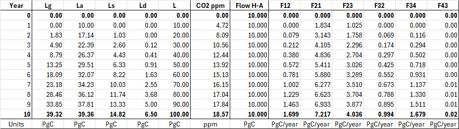
Here is table “Berry Carbon Flow Test” for discussion in our comments.
I request Ferdinand and anyone else who is contesting my calcuations to present your calculations for comparison.
We assume that the natural carbon cycle is at constant levels as shown in Figure 3.
With that information, we insert human carbon into the atmosphere at a constant rate of 10 PgC per year. Then we calculate annual time steps to see how much human carbon ends up in each reservoir each year.
This simple calculation is a way to compare our calculations because we keep human carbon inflow constant for each year.
The years run from zero to ten. All the L data are in PgC, and flow data are in PgC/Year.
Lg = land, La = atmosphere, Ls = surface ocean, Ld = deep ocean, L is the total PgC in the carbon cycle for each year. Ntice L increases by 10 PgC each year.
The CO2 ppm column simply converts the PgC in La to ppm.
Here’s how it works.
Year 0: 10 PgC is added to La, but you don’t see it until the beginning of Year 1.
Year 1: the 10 PgC in La produces outflows to Lg and Ls. We see the result in Year 2.
Year 2: the outflows from La have moved some carbon to Lg and Ls. Etc.
Notice that as La gets more PgC, its Outflow to Lg and Ls increase, etc.
While La increased by 7.14 PgC from Year 1 to Year 2, it increased by only 1.49 PgC from Year 9 to Year 10.
Also notice that as Lg and Ls get more carbon, they send carbon back to La.
Adjustment, Residence, E-time Compared
IPCC’s response times fail physics
Physics e-time has a precise definition. The IPCC times do not. In summary:
- Physics: e-time is the time for the level to move (1 – 1/e) of the distance to its balance level.
- IPCC: adjustment time is the time for the level to “substantially recover” from a perturbation.
- IPCC: residence time is the average time a CO2 molecule stays in the atmosphere.
IPCC defines “adjustment time (Ta)” as:
The time-scale characterising the decay of an instantaneous pulse input into the reservoir.
Cawley defines “adjustment time (Ta)” as:
The time taken for the atmospheric CO2 concentration to substantially recover towards its original concentration following a perturbation.
The word “substantially” is imprecise.
Cawley follows IPCC to define “residence time (Tr)” as:
The average length of time a molecule of CO2 remains in the atmosphere before being taken up by the oceans or terrestrial biosphere.
In summary, IPCC uses two different response times where it should use only e-time:
- When the level is far from its balance level (which can be zero), IPCC thinks e-time is an adjustment time because the level is moving rapidly toward its balance level.
- When the level is close to its balance level, IPCC thinks e-time is a residence time because “molecules” are flowing in and out with little change in level.
Figure A illustrates how e-time relates to IPCC’s adjustment and residence times.
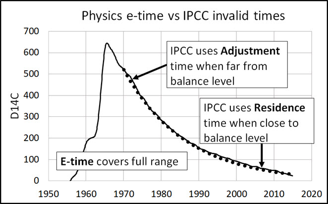
Figure A. E-time covers the full range of movement of level to a balance level. IPCC adjustment and residence times apply to only each end of the range.
IPCC, 2001: Working Group 1: The scientific basis. Appendix 1 – Glossary.
Lifetime
Lifetime is a general term used for various time-scales characterising the rate of processes affecting the concentration of trace gases. The following lifetimes may be distinguished:
Turnover time (T) is the ratio of the mass M of a reservoir (e.g., a gaseous compound in the atmosphere) and the total rate of removal S from the reservoir: T = M/S. For each removal process separate turnover times can be defined.
Adjustment time or response time (Ta) is the time-scale characterising the decay of an instantaneous pulse input into the reservoir. The term adjustment time is also used to characterise the adjustment of the mass of a reservoir following a step change in the source strength.
Half-life or decay constant is used to quantify a first-order exponential decay process.
The term lifetime is sometimes used, for simplicity, as a surrogate for adjustment time.
In simple cases, where the global removal of the compound is directly proportional to the total mass of the reservoir, the adjustment time equals the turnover time: T = Ta.
In more complicated cases, where several reservoirs are involved or where the removal is not proportional to the total mass, the equality T = Ta no longer holds.
→Carbon dioxide (CO2) is an extreme example. Its turnover time is only about 4 years because of the rapid exchange between atmosphere and the ocean and terrestrial biota.
However, a large part of that CO2 is returned to the atmosphere within a few years.
Thus, the adjustment time of CO2 in the atmosphere is actually determined by the rate of removal of carbon from the surface layer of the oceans into its deeper layers.
Although an approximate value of 100 years may be given for the adjustment time of CO2 in the atmosphere, the actual adjustment is faster initially and slower later on.
Ferdinand Engelbeen
August 8, 2025 at 3:14 am
Are you a robot? You keep making the same assertions without proof. Check this box if you are not a robot [].
Anecdotal data of seasonal mass transfers plus scientifically sounding, but invalidated formulas do not equal a coherent argument. Please show how the temperature dependency accounts for the change in CO2 over the whole Mauna Loa period using standard physics and no anecdotes or Magic Math.
Our Te models based on standard physics explain quantitatively within reasonable error the changes in atmosphere CO2. Our “theoretical world” matches the data. Your correlation-derived Tau depends on non-standard physical rules that you have yet to show the scientific basis for. They include your unscientific Temperature Dependency Principle, where temperature drives mass transfer with little concentration dependency, and net mass transfer being proportional to a difference between the current concentration and some equilibrium concentration in the past.
The Feely Formula, net mass transfer proportional to the difference between the current concentrations of pCO2 in the reservoirs, could be correct. But you have not shown how Tau is derived from that relationship. If that is wrong, please refer me to the appropriate date(s).
“Any calculations based on the 4 years turnover/residence time therefore have no connection with the real world” is another assertion without evidence. The Temperature Dependency Principle is simply an observation, not something you have derived from first principles. A Te of about 3 to 5 years was documented by most all scientists who published on this topic. It is only a subset that insist on the unverifiable unfalsifiable 50-year Tau.
Ferdinand,
Stephen P. Anderson, August 6, 2025 at 2:43 pm
“Yes, but I also know that these inflows (and the counter current natural outflows) are caused by temperature, bacteria, fungi, insects, animals,… largely independent of the CO2 quantity/pressure already in the atmosphere.
Most of these huge flows cycle in and out within a year. The only outflow that counts is the net difference at the end of a full year and that is caused by two items: one-way human emissions of FF use and the extra CO2 level/pressure in the atmosphere that causes more uptake than return from the natural sinks and sources.
See the difference in causes for the huge seasonal CO2 flows and the small overall result over a year I did send at August 6, 2025 at 9:04 am…………
Let’s just stick with the math. If natural emissions are around 100ppmv, then how can Te be more than about 4 years? I know Dr. Ed estimated 14CO2 Te at 16.5 years (he was just trying to show that the slowest Te is around 16.5 years based on the only data we have), based on that data, but all the other data suggest 12CO2 Te to be around 4 years. So, your argument is that the estimated 14CO2 Te of 16.5 years is an order of magnitude higher than 4 years and therefore your 55-year Tau (that keeps growing every year) must be correct? Is that your argument? If your Tau was legit and it keeps growing every year it would be a runaway situation.
Stephen Paul Anderson August 8, 2025 at 9:03 am
Dear Stephen,
In a recent comment, I updated my Te:
Te for Delta14C is 16.5 years
Te for 14CO2 is 10.0 years, which is my published Te for 14CO2.
Therefore, Te for 12CO2 is less than 10 years.
Also, for reference, IPCC’s natural carbon cycle data show its Te for 12CO2 is 3.5 years.
Jim Siverly, August 8, 2025 at 8:13 am
” Please show how the temperature dependency accounts for the change in CO2 over the whole Mauna Loa ”
No problem: per formula of Takahashi, based on meanwhile some 3 million seawater samples and Henry’s law for the solubility of CO2 in seawater for different temperatures:
If we assume (wrongly, as the real modern equilibrium is around 295 ppmv), that the equilibrium between ocean surface and atmosphere was established in 1960 at 315 μatm (~ppmv) at that time and the sea surface temperature increased with 0.6°C (HadSST3gl) then the increase in equilibrium (1960-2020) is:
(pCO2)seawater @ Tnew = (pCO2)seawater @ Told x EXP[0.0423 x (Tnew – Told)]
pCO2(2020) = 315 * EXP[0.0423 * (0.6)] = 323 μatm
Or an increase of 8 ppmv in equilibrium per Henry’s law. Not over 100 ppmv as observed, while humans emitted 170 ppmv of FF CO2 over the same time frame…
Vegetation acted as a net sink, as the O2 trends showed and also the increase of chlorophyll as observed by satellites as indication of increasing living organics…
“Anecdotal data of seasonal mass transfers”
The oxygen and δ13C measurements show a mass transfer between atmosphere and vegetation of over 120 PgC/season, half on daily, half on seasonal time scales. Since 1990 accurate enough for the O2 measurements to show the transfers. Nothing “anecdotal”, real, observed data. Here for the δ13C changes:
https://essopenarchive.org/users/529681/articles/606931-the-seasonal-cycle-of-%CE%B413c-of-atmospheric-carbon-dioxide-influences-of-land-and-ocean-carbon-fluxes-and-drivers
https://gml.noaa.gov/education/isotopes/c13tellsus.html
https://boris-portal.unibe.ch/server/api/core/bitstreams/3c99081b-6595-49db-b2ea-71fe69d79cd9/content
And many, many, many others that describe the seasonal (plant induced) δ13C changes.
The seasonal O2 changes are even more important, as these are far less mixed with O2 changes from the oceans than the opposite δ13C changes:
https://bluemoon.ucsd.edu/publications/ralph/3_Seasonal.pdf
https://www.tandfonline.com/doi/full/10.1080/16000889.2017.1311767#abstract
https://geoweb.princeton.edu/people/bender/lab/research_o2n2.html
And many, many, many others that describe the seasonal (plant induced) O2 changes.
Even the diurnal cycle is measured:
https://essd.copernicus.org/articles/15/5183/2023/essd-15-5183-2023.pdf Figure 15…
That are the large outputs of CO2 into vegetation which makes your much too short 4 years Te, largely independent of the actual CO2 level in the atmosphere…
Again: the main problem with Dr. Ed’s and your approach is the use of the turnover/residence time as an e-fold decay rate, while it is a simple division between the amount of CO2 in the atmosphere and the total outputs, not an e-time…
Dr. Ed, August 8, 2025 at 9:16 am
You forget the “dilution” of the 14C “fingerprint” by the 14C-free FF emissions and the return of “old” 14C level CO2 from other reservoirs, which make the 14C decay rate faster (not slower) than for 12CO2.
And the IPCC explicitly rejects the use of the turnover time T as an e-fold decay rate Te…
Stephen Paul Anderson, August 8, 2025 at 9:03 am
“Let’s just stick with the math. If natural emissions are around 100ppmv, then how can Te be more than about 4 years?”
The turnover/residence time is about 4 years. That is the simple formula:
RT = level / output.
No matter if the output is caused by the level or any other process, independent of the level.
In the real world, 95% of the outputs is caused by processes which are independent of the CO2 level in the atmosphere and only 5% are level dependent.
That makes that Dr. Ed’s and Jim’s calculations, based on an exponential decay rate of 4 years is completely at odds with the real world, because Te may not be set equal to the RT of 4 years, as that are two completely separate items.
With a Ta/Tau of around 50 years, the decay of our FF emissions is not fast enough to remove all FF in the same year as emitted, but when FF emissions are halved, that would stop the CO2 increase in the atmosphere and with a full stop, after 35 years (the half life) the extra CO2 drops to around 360 ppmv, after 70 years to 325 ppmv,…
Ferdinand Engelbeen August 8, 2025 at 9:51 am and 10:07 am
Dear Ferdinand,
Contrary to your claims, my model calculates what you call “dilution” of 14C by 14C-free FF emissions, and the recycling of 14C from other reservoirs.
By contrast, your model calculates nothing. It can’t because you have no mathematical formulation of a carbon cycle.
The outflow (that you call decay rate) of 14CO2 cannot be faster than the outflow of 12CO2 from any reservoir.
My Te definition has no dependance on anything the IPCC writes. I formed it from the way systems models are supposed to be formulated, with is fully described in the WIKI reference that you provided.
You wrote, “In the real world, 95% of the outputs is caused by processes which are independent of the CO2 level in the atmosphere and only 5% are level dependent.”
You have made that same claim over and over again. But you have failed to show how your claim changes my (2) that Outflow = Level / Te
While no carbon cycle data are exact, IPCC’s data for its natural carbon cycle is a valid reference for “the real world.” It is the place where all carbon cycle models should begin.
My Te replicate IPCC’s natural carbon cycle. Your claimed carbon cycle cannot replicate IPCC’s natural carbon cycle or any other data that you have presented to this extensive discussion.
So, your claim that Te cannot be set to 4 years, is invalid because it is contradicted by IPCC’s data.
You claim: “With a Ta/Tau of around 50 years, the decay of our FF emissions is not fast enough to remove all FF in the same year as emitted, but when FF emissions are halved, that would stop the CO2 increase in the atmosphere and with a full stop, after 35 years (the half life) the extra CO2 drops to around 360 ppmv, after 70 years to 325 ppmv,…”
No data, used properly, supports your claim. IPCC’s own carbon cycle data prove your claim is wrong.
Ferdinand, it is time for you to stop recycling your invalid claims over and over again, when they contradict both physics and real data.
Ferdinand Engelbeen
August 8, 2025 at 9:43 am
It seems what you have shown is that temperature alone cannot account for the measured rise in CO2 between 1960 and 2020. What you have not shown is how much FF contributed any known amount of that rise, because you rely solely on Magic Math.
Are we to guess how your O2 and 13C references allow you to arrive at the conclusion, “That are the large outputs of CO2 into vegetation which makes your much too short 4 years Te, largely independent of the actual CO2 level in the atmosphere?” I have no clue how you get that.
You see a problem with our approach, because you have invested so much into your approach that you can’t let it go.
The latest kerfufal is the administrations declaration of abandonment of the OCO satellite. The activists siting the quality of the measurements, youth and good condition of the vehicle, and the relatively low cost of maintenance and data gathering. The administration citing the lack of utility for the data. I am a died in the wool proponent of getting the most out of what you have and watching for alternative uses for my tools and information. Has anyone that is participating in this discussion on Dr. Ed’s site analyzed the OCO data to see if it can support either side of this discussion ? My brief introduction to that data revealed that the measured sources of CO2 do not align with the model distribution. The graphic I saw showed barely increased concentration in populated areas except for China. My take on it was that the overwhelming majority of the measured emissions are natural and the human contribution could easily be lost in the noise but that was from just a visual review.
Dr. Ed, August 8, 2025 at 11:12 am
“Contrary to your claims, my model calculates what you call “dilution” of 14C by 14C-free FF emissions, and the recycling of 14C from other reservoirs.”
Yes, your calculations for the 14C decay includes the dilution, but you forget that there is no such dilution is for the decay of a bulk 12/12CO2 injection, thus that the decay rate for a 14C injection is much faster than for a 12/13C injection. Not slower…
“But you have failed to show how your claim changes my (2) that Outflow = Level / Te”
If there is hardly any connection between Level and Outflow, then Te doesn’t tell you anything about the fate of an extra injection of CO2 of whatever source in the atmosphere…
RT/Te is based on outputs alone.
Ta/Tau is based on the difference between inputs and outputs.
The first shows how fast the CO2 mass is moving through the atmosphere.
The second shows how fast an extra CO2 mass injection is removed out of the atmosphere.
From the first you can’t calculate the removal rate of an extra CO2 mass injection, only how fast an individual CO2 molecule is replaced by a CO2 molecule from another reservoir.
“My Te replicate IPCC’s natural carbon cycle.”
Your Te violates the carbon mass balance: if human CO2 is rapidly distributed into oceans and vegetation, then the observed increase in the atmosphere must come from the same reservoirs, which makes that the total increase in atmosphere + oceans + vegetation is much larger than from the FF emissions…
“No data, used properly, supports your claim. IPCC’s own carbon cycle data prove your claim is wrong.”
Even from the start of this discussion, I have sent the calculated CO2 increase with the 50 year Ta/Tau that near perfectly match the Mauna Loa data… And that obeys the carbon mass balance…
https://www.ferdinand-engelbeen.be/klimaat/klim_xls/Berry_fluxes.xlsx
The IPCC’s overall Ta is even worse, going to hundreds of years for a part of the FF emissions…
Jim Siverly, August 8, 2025 at 12:38 pm
“What you have not shown is how much FF contributed any known amount of that rise”
It is pretty sure that all FF emissions are for 100% directly into the atmosphere: as mass and as isotopic composition.
As we measure the change in CO2 mass of the atmosphere and the change of its isotopic composition, we know that about half the FF emissions as mass per year are removed and about 2/3 of its isotopic composition are replaced by CO2 from other reservoirs. That means that FF emissions are fully responsible for the increase in mass and the decrease in isotopic ratio. Only Magic Math can give a different outcome…
“Are we to guess how your O2 and 13C references allow you to arrive at the conclusion, “That are the large outputs of CO2 into vegetation which makes your much too short 4 years Te, largely independent of the actual CO2 level in the atmosphere?” I have no clue how you get that.”
Sorry, but I thought it would be clear from the IPCC’s scheme in Dr. Ed’s Figure 2, that the largest flows are bidirectional and near equal.
Dr. Ed’s and your Te of 4 years only looks at the level in the atmosphere and the output level, but that doesn’t say anything about the cause(s) of the output(s) neither of the input level.
In the case of large cycles within a day/year, the output level doesn’t change at all if input and outputs are equal, thus without any change in level, while the output still is high and the residence/turnover time still is 4 years.
If there is any extra input, of whatever source, then only the difference between inputs and outputs tells you what the real decay rate is and that is Ta/Tau, no matter the height of the inputs and outputs…
If the outputs are not 100% dependent of the level in a reservoir, then the decay rate Te never can be equal to the residence/turnover time. That is the crux of the matter in this whole discussion…
“You see a problem with our approach, because you have invested so much into your approach that you can’t let it go.”
I only see that your approach is based on a model that implies that a change in level causes an equal change in output, while the data show that a 50% change in level only causes a 33% change in output towards the oceans and a meager 13% towards vegetation. Which proves that your model is wrong…
DMA, August 8, 2025 at 5:12 pm
My impression is that the data are not as accurate as they have expected, from the beginning on.
That being said, there are several problems with the CO2 releases that they underestimated: the OCO measurements are only within sunlight, while most emissions out of vegetation are during the night.
https://ocov2.jpl.nasa.gov/science/measurement-approach/
And human emissions are quite small and fast mixed in the total atmosphere. A 5 ppmv increase over a year is 0.15 ppmv / day change. The accuracy of the measurements is 0.8 ppmv over land and 0.5 ppmv over water. Only in tight populated and industrialized regions, that would be measurable…
But stopping these measurements would be a loss of knowledge…
As an end of this discussion, my last contribution:
How much carbon is in a reservoir is not important, as long as it stays there.
How much carbon is exchanged between reservoirs is not important, as long as in and outs are equal.
Only the difference between ins and outs changes the carbon content of a reservoir.
The 4 years Te only looks at the second part.
The 50 years Ta/Tau looks at the last part…
Dr. Ed,
Sorry, I didn’t realize you had a new estimate for 14CO2 Te. When you have mass that is such a minute part of the total mass of the atmosphere, it must be difficult to get an accurate concentration. Also, Ferdinand does not understand that the balance level is some level in the future. It is not the real-time level, but is set by the real-time emission. He either refuses to accept or to understand the continuity equation, which is nothing more than a mathematical description of the natural process.
Ferdinand,
Thanks for the debate. You’ve been a good sport. I do agree with you about one thing. CO2 is good.
Dear Dr. Ed,
I finished a first draft of a one-compartment model for 14C that simulates Figure 2 of Schwartz et al. 2024. I started with the CO2 model where I generated an exact fit to the Mauna Loa data using a solution to the differential equation dC/dt = Eh + En – C / Te. To test my model, I first established equilibrium conditions that would have been in effect prior to 1750. Assuming the atmosphere contained 600 PgC 12C and 600 Kg 14C, I found a 5-year e-time held both amounts constant. Equilibrium for 12C occurs, because no change in net CO2 occurs with the annual exchange of 120 PgC. Equilibrium for 14C occurs because for every 7.5 Kg 14C produced annually from cosmic ray reactions with N2, another 112.5 Kg enters the atmosphere from the 600 PgC emitted by the reservoirs. The reservoirs, in turn, received 120 Kg 14C from the atmosphere. I don’t remember if I tested other e-times, but whatever e-time is assumed requires assuming a lower concentration of 14C in the reservoirs than in the atmosphere, otherwise there would be no equilibrium.
Next, I incremented my spreadsheet as before with an amount of additional CO2 to supplement FF CO2 and maintain the match to Mauna Loa data. The 14C incremented with the same differential equation as 12C such that by 1950, delta14C matched the measured data. In other words, the FF emissions diluted 14C somewhat for over two centuries and the spreadsheet followed that accurately.
Beginning in spreadsheet row for 1955, I manually added enough 14C each year to approximate the rise in 14C from the bomb tests up to the peak in 1966. At that row, I returned to the previous formula operating with the original e-time of 5 years. As might be expected, 14C depleted much faster than the known data. Assuming an additional amount of 14C was being returned to the atmosphere from the newly 14C-enhanced reservoirs, I added an exponentially decreasing amount of 14C to the ongoing increase from the pre-bomb influx formula. Logically that additional amount would be expected to decrease as the bomb carbon dissipated into the deep ocean and returned 14C to its pre-bomb level.
https://www.dropbox.com/scl/fi/qqtwvp85x47fqgxmou2wd/one-compartment-14C-model.png?rlkey=es0h0rfb2mg2xbmd685r97mkx&dl=0
My graph shows two curves for each of the two ways of reporting 14C. The lower curve of each pair represents a formula that avoided including any 14C from the FF carbon emissions. In other words, without distinguishing between natural and FF emissions, the 14C is over counted.
More importantly, the formulas employed to generate the graph reinforce the principles you expound and have demonstrated with your model. There is only one e-time needed to explain the dispensation of bomb 14C. The decay profile is akin to a removal “wave” from the atmosphere impeded by an “echo” of 14C returning from the reservoirs. That phenomena is integrated into the normal exchanges between the atmosphere and the reservoirs resulting in the appearance of an e-time longer than the usual four or five-year e-time.
For the years prior to the bomb tests, the spreadsheet maintains a preindustrial equilibrium and increments 14C accurately using a single formula based on multiple inputs and a constant output rate into and out of the atmosphere to and from other reservoirs. The injection of 14C in the 50’s and 60’s cannot be characterized by a one-compartment model without the manual additions and manipulating a decay profile that matches data. However, those additions and subsequent relaxation of 14C should be adequately described using a two-compartment model similarly derived.
Dr. Ed,
While anticipating push-back on my last comment, I was catching up on popular climate news and came across this at drroyspencer.com: https://www.drroyspencer.com/2025/07/some-thoughts-on-our-doe-report-regarding-co2-impacts-on-the-u-s-climate/
“That same morning I [Dr. Roy Spencer] was called by a particle physicist who heard all of this news [about the Remote Sensing journal editor forced to resign for publishing a Spencer paper] and said something to the effect of, ‘What’s wrong with you climate guys? We have people who believe in string theory and those who don’t, but we still work together.’ We both laughed over the divisive nature of climate science compared to other sciences.”
That struck me as a good summary of this debate. “Climate” science adopts principles not shared by mainstream science. Need I delineate them?
Jim,
From all your work, what did you calculate for e-Times for 12CO2, 13CO2 and 14CO2? Pretty much the same as Dr. Ed’s calculations? Thanks
By the way, this page is a great reference page for future.
Jim,
One of my on-going arguments on Dr. Spencer’s site is that in my view the lapse rate falsifies the GHE. For instance, according to GHE, if greenhouse gases were eliminated from the troposphere, then the troposphere becomes isothermal. My argument is you’d still have a difference in temperature at altitude based on hydrostatic pressure, lapse rate.
Stephen Paul Anderson
August 12, 2025 at 1:21 pm
Stephen,
My Te for 14C is the same for 12CO2, in this case 5 years. However, that maybe somewhat flexible. Most of my time was spent making sure I had equilibrium conditions prior to the introduction of FF and bomb emissions. Until the bomb tests, those e-times had to be the same because of the equivalence principle. After bomb testing, the equivalence principle still applies but the “equilibrium ratio” was thrown off. Then the superposition principle kicks in. That requires a different formula operating. A decay function is superimposed on the normal Te function. The decay e-time I used for the excess amount (the “echo”) emitted to the atmosphere is 15 years, but I am not sure how accurate that is. I should go back and try 16.5 years, because that is what the observed decay rate is.
August 12, 2025 at 1:30 pm
There has been much discussion of what the troposphere would become without IR-absorbing gases (I detest the use of GHG terminology). If you are arguing no change in lapse rate, I agree with you. On which post is that discussion happening?
Jim,
We post on drroyspencer.com. Not much is happening now. It is mostly anti-Trump comments-his takeover of D.C., and Dr. Spencer’s DOE report. They should have had Dr. Berry included on that committee. Thanks for your input on Te. Do you have a webpage where you post your charts?
Stephen,
I adjusted my decay rate to 16.5 years and it reduced the 14C/12C curve to below the observed curve. And then I changed e-time to 5 years and that restored almost a perfect fit.
Also, I have not done any 13C work, but I’m looking into it now. I don’t have a webpage, but I am thinking of writing a paper on the results. It depends on whether anyone else has already done it.
Jim,
I don’t know why I am responding to your 14C analysis, since you don’t even accept the basic fact that data and a little accounting clearly show natural processes are removing carbon from the atmosphere, not adding it. But I will, because there are too many obvious problems with it.
1. Although you generated a 14C concentration curve somewhat similar in shape to the data following the bomb pulse, it certainly does not match the data. The data never gets much below 500 amole per mole before rising, but your two curves bottom out around 400 and 425.
2. I don’t understand why your “mole fraction all CO2 and “mole fraction no FF CO2” curves are different. I trust you are aware that FF CO2 contains negligible 14C, but perhaps you are not.
3. You should look at Figure 4 in the Schwartz paper as well as Figure 2. It shows how 14C moved between various reservoirs (stratosphere, troposphere, biosphere, oceans) after the nuclear testing.
4. You will note from that same Figure 4, that the nuclear testing put about 100 Kmoles of 14C into those reservoirs, and most of it is still there. What time constant do you think determines its removal? Please don’t say four years.
5. You wondered if anyone else had tried an unconventional explanation of the 14C history, as you have done. Harde and Salby did. They realized, unlike you or Ed, that they had to explain an increase in the total amount of 14C in the fast cycle reservoirs. So they postulated new sources which were not credible. See the Appendix in https://scienceofclimatechange.org/wp-content/uploads/Andrews-2023-Clear-Thinking-about-Atmospheric-CO2.pdf Their explanation was aimed at suckers, not scientists, and that is why I earlier expressed my disdain for the (deceased) Murray Salby. He was unethical in his science as well as in his management of grant money.
David,
Thank you for the opportunity to clarify points your questions raise and the benefit your criticisms bring toward improving my model.
First of all, papers like one you cited (Graven et al. 2020) explain how natural processes are removing carbon from the atmosphere AND adding to it. It’s the basis of what is meant by disequilibrium fluxes.
1. It’s true that I am short on how much 14C my spreadsheet predicts following the bomb pulse. I will need to add additional amounts in the lead up to the max around 1966. I will do that and also compare my gross 14C amounts added to what others have published.
2. In both cases, the upper curves represent the calculation that results if one doesn’t take into consideration that FF emissions contain no 14C. That was to highlight the magnitude of the difference FF carbon makes in the whole scheme of things. The lower curve represents the true 14C calculation to within whatever degree my formulas and inherent assumptions are correct.
3. I will generate a Figure 4 type graph from whatever information I can get out of my model. That would be a logical step toward model validation.
4. My one-compartment model only includes the 4-year removal rate constant, because that is the only one necessary. Nature didn’t suddenly change to accommodate bomb carbon. The other rate constant (now 16.5 years) in my model is inferred from what would be necessary to account for the back flux from the first, second, third,…, nth generation return of 14C due to disequilibrium isoflux. However, that inferred rate constant also includes contributions for 14C originally in land and ocean reservoirs from post bomb treaty testing (underground and in the ocean) and subsequently from nuclear energy production. I say inferred, because a one-compartment model can’t handle the contributions from the reservoirs without manual splicing in the second compartment contributions. Everyone agrees, except maybe you and Ferdinand, that reservoirs were adding more 14C to the atmosphere than the atmosphere was removing.
5. I reserve a response on the Harde and Salby 14C history until I do a thorough review of the appropriate papers.
Thanks again for your questions.
While tweaking my model to get closer to the Schwartz data, I noticed that changing e-times throws off the C12 and 14C equilibration that was assumed to have been established prior to the perturbations introduced by FF and bomb testing. Some, if not all, of the starting variables are interrelated, such as the equilibrium ratio of 14C/12C, a natural e-time for removal, and the starting CO2 concentration. This is an important point, because everyone assumes it was around 280 ppmv. But nature has been trying to establish an equilibrium much before this millennium. In that case, some initial disequilibrium values should be considered acceptable.
Now let’s consider your point 5. where you accused Dr. Ed of not understanding the difference between DC14, the 14C/12C ratio, and molecular 14C. In Berry 2019, he refers frequently to 14C data and equates it to Hua DC14 data. Therefore, I don’t view that as problematic. His whole point was to illustrate that the IPCC model could not do what his model does, replicate the Hua data. Dr. Ed has already admitted mislabeling the graphs and that should be enough said. Also, similarly, nothing other than poor labeling in the Harde 2019 paper indicates him being confused over absolute 14C versus the 14C/12C ratio.
Back on July 10, 2025 at 6:41 pm (https://edberry.com/co2coalition/comment-page-3/#comment-112521), you postulated, with all other things equal, that a bomb experiment would result in 14C decaying to normal in about a decade. Have you ever tried modeling that?
David Andrews
August 13, 2025 at 9:22 pm
I’m working through your paper and came to the analogy in section 3.5 of the couple putting and taking from an account. I have seen this often and think a better analogy would be a bank with many clients some just deposit others just withdraw many do both. The account at the end is just as definitive as the couples’ account – the net increase is less than the deposit record of one client that took no withdrawals. How can the bank know the increase is due to that client? Just like CO2, without some analysis of flow the only valid statement is “That source likely contributed to the increase.”
Jim,c
What starting CO2 concentration works best for your model? No one knows what the CO2 concentration was in 1750.
Jim,
You ask: “Back on July 10, 2025 at 6:41 pm (https://edberry.com/co2coalition/comment-page-3/#comment-112521), you postulated, with all other things equal, that a bomb experiment would result in 14C decaying to normal in about a decade. Have you ever tried modeling that?”
There is not much to model. By the assumption of the thought experiment, everything is in equilibrium until the abrupt injection of a part per trillion of 14C into the atmosphere. That does not stimulate plant growth. That does not appreciably increase ocean carbon content. But it does create an isotopic disequilibrium since the atmospheric 14C level was doubled. The balanced exchanges which are maintaining the overall carbon equilibrium then move 14C from the atmosphere to the land/sea reservoirs, until the isotopic difference is erased. Think MIXING, not ABSORPTION, with no change in carbon levels or flow rates beyond a part per trillion. (Of course this mixing is our “disequilibrium isoflux”.) That is what happened after the real-world experiment in the 1950’s and 1960’s, though the background processes were not perfectly balanced as in the thought experiment. The data from that period tells us that the mixing time scale is about a decade.
I can tell you are struggling with your model because you are wrongly changing carbon levels on a short time scale. Ferdinand tried to tell you that the mixing time scales and level-changing time scales are different. Perhaps you will learn from your struggles.
DMA,
You ask: “the net increase is less than the deposit record of one client that took no withdrawals. How can the bank know the increase is due to that client?”
My first answer would be that if the client that took no withdrawals had also not made any deposits, then the total bank deposits would have decreased. (I have to be careful how I say this, since to a bank, a deposit is a liability and a loan is an asset.)
For carbon and the carbon CYCLE, I think it is better to think about the history of the carbon in any particular stream and ask yourself where it came from and how stocks are changing. Sure, oceans are mostly outgassing carbon in the tropics, but they are mostly absorbing it nearer the poles. The carbon in that outgassing stream in the tropics was not that long ago in the atmosphere. Unless you had evidence that ocean carbon content was decreasing (of course in fact it is increasing), you cannot sensibly separate the tropical ocean outgassing from the polar absorption and call the oceans a source. The same goes for the growing biomass. Trees don’t make carbon, they just borrow it. If the biomass is bigger now than a century ago, then biological processes must be removing carbon from the fast cycle, not adding it. On the other hand global fossil fuel reserves are DOWN. The decrease in carbon in underground reserves accounts for the increase in carbon in the atmosphere, and in the other reservoirs.
Stephen P. Anderson
August 15, 2025 at 7:20 pm
To a first approximation, it doesn’t matter what the CO2 concentration was in 1750. However, you have to have a model that is consistent with maintaining an equilibrium at some distant past time. Then going forward, that model has to correctly match 14C and Mauna Loa data. What I’m finding is I can start with any e-time within 4 and 10 years (although not necessarily limited to that range) and add an exponential amount of additional emissions that will give me a good match to the Mauna Loa data. I have not extended that to 14C data yet. More on this later. The link below is a modified 1-compartment spreadsheet model that illustrates what I’m finding. You can experiment yourself with alternative e-times and changing the exponential parameters to determine the determine the appropriate amount of additional emissions. Warning: This can be time-consuming, but worth the exercise in seeing how the exponential affects the fit. Hint: one parameter shifts the curve and the other bends it.
https://www.dropbox.com/scl/fi/4idfv1xf7omq02g66pwhl/CO2-model-changeable.xlsx?rlkey=7b3i20ajx076j54yke6r7jpk0&dl=0
As for starting concentrations, the model will move to its balance level depending on the e-time. One can get to the balance level immediately by entering a starting input rate = balance level / Te.
David Andrews
August 15, 2025 at 10:04 pm
Dear David,
While being indebted to you for forcing me to look at the other papers aligned with Dr. Ed, I can assure you I am not learning from your and Ferdinand’s simple math and mixing time scales and level-changing time scales. Your disinterest in modeling is telling and might indicate that you are still struggling with understanding the intricacies introduced by Dr. Ed et alia, if not accepting them.
Getting back to Harde and Salby 2021 (August 13, 2025 at 9:22 pm, point 5.) I was pleasantly surprised to see Harde and Salby 2021 proposing an unconventional explanation of the 14C history requiring additional CO2 from non-FF sources. The authors’ beta coefficient accomplishes the same result as my exponentially increasing additional emissions, although they itemize where the additions come from, namely background, asymmetry, temperature, and re-emission. Those currently amount to 3, 27, 3, and 59 ppmv/year, respectively. In my view, re-emission is a misnomer. It basically accounts for the remaining emissions required to make the evolution curve match the Mauna Loa data. Am I wrong? Furthermore, Harde and Salby claim that Tau_eff for 12C was determined independently of its determination from 14C data. I’m inclined to disagree with that. One can’t extricate a Tau determined from 14C when 14C and 12C are both inherently linked by the equivalence principle. The differences in 14C and 12C dispensation is due to the bomb testing injecting an anomalous amount of 14C into the system. That creates differences in their emission and absorption rates but not a difference in rate constant.
Continuing from what I was explaining to Stephen, I find any removal rate constant between 0.1 and 0.25 will match Mauna Loa data with the appropriate emissions added. Do you agree their re-emission term is simply an additional amount needed to supplement the additions contributed by background, asymmetry, and temperature?
Jim,
I will let you believe that the 14C errors of Berry and of Harde and Salby prior to 2019 were mere clerical errors, but they were not. They were fundamental errors critical to the wrong arguments being made. They were the kind of errors that peer review catches. I have nothing to add to my critique of Harde and Salby’s failed attempt to patch up their theory by inventing an unrealistic background. You are the perfect mark for their scam. They are telling a gullible non-scientist what he wants to hear.
Mainstream atmospheric science has never had a problem understanding and interpreting the 14C data. Ed still scoffs at disequilibrium iso-fluxes (DIF), presumably because they fooled him into thinking that his calculation of the composition of the present atmosphere meant something. His analysis in the paper critiquing the CO2 Coalition at the top of this thread shows he still does not understand the Seuss paper from the 1950’s.
Let’s get back to the main question: why is atmospheric CO2 increasing? I am very skeptical of your hypothesis that natural emissions have had a huge increase since 1750, but it is not really a hypothesis. It is just a parameter in a curve fitting exercise that explains nothing. Your spreadsheet inputs fossil fuel emissions data and Mauna Loa data, and so correctly shows a positive net global uptake. Natural processes are removing more carbon from the atmosphere than they are adding in your world as well. I rest my case that human emissions are the culprit. After all your spreadsheet work, what is your argument that natural processes are responsible?
David,
My hypothesis is that some of the rise in CO2 is due to FF emissions and the rest are natural emissions which to some degree are caused by human activity. My justification for arguing that additional natural emissions are necessary comes from failing to find a match to the Mauna Loa data using only industrial emissions. I found that I can achieve good fits with a range of e-times, but only an e-time of four to five years is consistent with the IPCC report that natural emissions are about twenty times those of the industrial emissions.
I am still working through your critique of Harde and Salby 2021 and I think you have some valid complaints, but I give them major credit for incorporating the seasonal variation of CO2 and the 14C oscillations immediately after the bomb testing peak that reflect annual re-enrichments of tropospheric 14CO2 from the stratosphere. One has to admit how cool those are. Those enhancements are basically superimposed on the general evolution of increasing CO2.
Still the question remains, what else drives the CO2 rise, assuming industrial emissions do not account for all of it? In my mind, it’s obvious. Let me try to explain why you don’t see it. I think you, like Ferdinand, ascribe to the view that mass transfer rates are not entirely proportional to concentration differences. Please correct me if I am wrong. To appreciate where I and others are coming from, one must recognize the concentration-dependent bidirectional relationship between the atmosphere and its adjacent reservoirs. The general relationship is dC/dt = – k1*[A] + k-1*[B] where [A] and [B] represent the concentrations of carbon in the atmosphere and in any given reservoir, respectively. Each reservoir has a unique set of forward and reverse rate constants, but in a simplistic general sense k1 and k-1 comprise an average of all exchanges between the atmosphere and the reservoirs. Without an appreciation of this generally true physical phenomenon, you and I will never come to a meeting of minds.
So, if industrial emissions do not accumulate in the atmosphere as you concede, then what causes the rise? All of the players involved in this discussion agree that temperature is only partially responsible. Harde and Salby appear to suggest the asymmetric seasonal change accounts for another part of the rise. Unless I missed it, that is a result of an unexplained cause, not a cause in itself. I do appreciate the need for additional emissions to get a Mauna Loa data fit. Not having thoroughly understood your critique of their “background” scenario, I will move on to the other possible emission sources that have not been mentioned, one from land and the other from the ocean.
Going back to the dC/dt equation, there must be additional emissions coming from somewhere other than industrial emissions, otherwise a near equilibrium would be hovering just above 300 ppmv according to my spreadsheet model. In other words, [B] has been gradually increasing. One obvious possibility is the increased emissions created by an 8 billion population increase. Land use change has probably been significantly under counted. The other possible source of inflated [B] could be an incorrect interpretation of the ocean concentration making its effect less than recognized. I could break that down further, but I would like your take on my other responses first.
I have still been waiting to see the final version of “CO2 Coalition’s not so Golden Science” so that I can circulate it to a climate discussion group. Did I miss it? Thanks.
Jim,
I have spent little time myself worrying about time constants, as the carbon conservation (mass balance) argument does not require that detail. That is the typical beauty of using conservation laws. Your term (Magic Math!) is appropriate.
Still, I think I know what your main problem is. You have pointed to two things that worry you about your spreadsheet results:
1. If you only consider the industrial emissions, your spreadsheet yields too small a rise.
2. You need to postulate increasingly large natural emissions to keep up with the measured (Mauna Loa) atmospheric accumulation of CO2.
Both of these problems would be solved by the use of a much longer time constant.
Some modelers studying problems such as “what exactly happens after net zero” combine the atmosphere and surface ocean into one reservoir. After all, it takes a year or two for the northern and southern hemisphere atmospheres to mix, almost as long as for the atmosphere to mix with the surface ocean. So if you want to study what happens on decadal time scales, you might as well lump them together. Now the question becomes, “how fast do transfers between the atmosphere/surface ocean and the deep ocean occur?” The answer is, much longer than 4 years (maybe 50 years, maybe a century). But those processes are essential for understanding the growth of atmospheric CO2, as the surface ocean CO2 is growing with it. Information about those slower processes is NOT contained in the 14C bomb pulse data.
The real-world carbon cycle is complicated. You are not the first to try to capture the whole thing with one time constant. You won’t be able to do it and others couldn’t either. You are too optimistic about what you can get out of a one box model. But you still can use Magic Math to figure out what is causing the rise.
David,
You are suffering from Wizard of Oz syndrome. Never mind the time constants behind the green curtain, just click your heals together and Magic Math will get you back to Kansas. In the real world using real physics you will never get a model to fit real data with the much longer time constant you suggest.
I agree that transfers between the atmosphere/surface ocean and the deep ocean are essential for understanding the growth of atmospheric CO2, but no one has demonstrated how longer e-times for the ocean require any longer e-time for the atmosphere. And 14C bomb pulse data Information can only improve our understanding about those slower processes.
I finished your critique of Harde and Salby 2021. Although I am troubled by their conversion of a four-year e-time into a ten-year effective one, I don’t find anything unreasonable about their model. At worst, one might say it is only partially quantitative with qualitative assumptions filling in the gaps. I think it’s not unreasonable to say their analysis is somewhat better than your 100% qualitative isoflux-based analysis. You are quick to point out problems with the models of others without having one of your own. It’s time you converted your qualitative arguments into a dC/dt = something model.
At the top of page 41 of your “Clear Thinking about Atmospheric CO2” paper, you wrote, “To transform the red curve in Figure 2 to the green curve, their solution is to postulate new sources of atmospheric 14C that started after about 1964.” That is confusing because Harde and Salby were not transforming red to green. They showed how their model explains the known red curve data. At first glance, in other words without having run the numbers yourself, why would you deem “new” sources of 14C necessary? After all, the main reason for the red curve differing from the green curve is the additional bomb 14C that tracks the atmosphere’s rise in CO2. The green curve only accounts for the bomb pulse. The red curve accounts for additional 14C coming along with the 100 ppmv increase in CO2 since 1965. The only reason to postulate “new” sources of either 14C or CO2 is, because without it, one cannot formulate a model that includes proper physics and explains all the data.
Jim,
The carbon conservation argument is rock solid. It was cited in the Trump administration’s Climate Assessment Report, where it was about the only thing they got right. You have never said what you don’t understand. Go ahead, ask me a question about it. Ed’s approach over the last several years has been to misrepresent it, then argue against the straw man he created, then block posts that counter his points. (I thank him for not blocking me these last couple of months.)
I reviewed what I wrote about Harde and Salby concocting a new background when they realized the concentration curve was not the same as the Delta14C curve as they had previously thought. I stand by what I wrote. It was them, not me, that postulated the unreasonably large new radiocarbon sources. Perhaps you have to read all the papers to understand the history.
Perhaps I should not be surprised that you are sympathetic to the Harde and Salby curve fitting approach. All that you have done is invent numbers to fit the Mauna Loa rise, as they did to fit the 14C concentration curve. Your increasing natural emission numbers are no more credible than their cosmic ray flux increase, and they are required for similar reasons. Yet you call your approach “proper physics”. Sorry. I think you need to go back to school.
David,
I am not the one being childish. It’s you that defends a simplistic view that cannot explain how only a few percent of the atmosphere containing FF emissions causes all of the rise. And you have the gall to ask me what I don’t understand about it! Boy, that is some kind of hubris.
You scoff at Harde and Salby’s cosmic ray flux increase which is based on real data and fills in a part of their model that didn’t fit all the data. You decry our attempts to use proper physics and yet have no model of your own. You claim carbon conservation which isn’t even applicable since you and the rest of your simple math advocates can’t account for all the carbon you claim to have conserved.
Good grief, Charlie Brown.
Since your attacks on me, Harde/Salby, and Dr. Ed are farcical, would you care to be specific about what else you think the Trump administration’s Climate Assessment Report got wrong?
Dr. Ed,
In the last paragraph of the Overview Section 1.1 on page 4, you have, “Neither Lindzen, Happer, nor Koonin (2021) have made any public arguments to support or deny their belief in H(1).”
Check this out: https://www.sealevel.info/Happer-Koonin-Lindzen.pdf
The last paragraph on page 20 begins with, “Growing human emissions have increased the atmospheric concentration of CO2, from about 280 ppm in 1900 to just over 408 ppm today. The long atmospheric lifetime of CO2 and the roughly constant airborne fraction mean that this concentration growth is proportional to the cumulative human emissions.”
That paragraph ends with, “CSSR Figure ES.3 shows that all global emissions must cease beyond 2075 if human influences are to be stabilized at allegedly “safe” levels.”
Figure ES.3 can be found on page 16 here: https://www.nrc.gov/docs/ML1900/ML19008A410.pdf
It’s no wonder CO2 Coalition includes Happer and Lindzen as supporting the mainstream climate view of H1.
I’m referring to a previous comment by David Andrews. If I understand correctly, the so-called “mass balance” argument (repeated like a parrot by the indoctrinated AI Grok) goes something like this: humans emit 38 billion tons (Btons) of CO₂ annually, while the observed increase in atmospheric CO₂ is only 19 Btons per year. Since 19 is less than 38, the conclusion drawn is that Nature must be a net emitter and therefore cannot be contributing to the rise in atmospheric CO₂.
This reasoning, however, is fundamentally flawed.
When we examine both natural and human carbon flows, we recognize that emissions in a given year are also partially reabsorbed by natural systems. The carbon cycle—whether considering human or natural contributions—is defined by a continuous process of emission followed by absorption. The net change in atmospheric CO₂ concentration depends not only on gross emissions, but also critically on how much is reabsorbed.
With this in mind, the correct “mass balance” equation should be expressed as:
DC = HE + NE – NA
Where:
• DC = Annual change in atmospheric CO₂
• HE = Human emissions
• NE = Natural emissions
• NA = Total absorption by nature
Since nature absorbs portions of both human and natural emissions, we can further detail NA as follows:
NA = HE* fh + NE*fn
Where:
• fh = Fraction of human emissions absorbed annually
• fn = Fraction of natural emissions absorbed annually
Combining these equations allows us to isolate NE:
NE = [DC – HE*(1 – fh)]/(1-fn)
The flawed mass balance argument assumes fh = 0 and fn = 0, which leads to NE = DC – HE. Substituting the proposed numbers, this implies:
NE = 19 – 38 = -19
This would mean nature actually reduces atmospheric CO₂—contrary to the conclusion that it cannot contribute to the increase.
But this scenario ignores reality: both fh and fn are undeniably greater than zero. When this is correctly accounted for, NE can easily exceed zero and, in fact, become dominant in the balance.
I refer to this oversimplified and misleading argument as “Cawley’s Trick,” named after the author who issued a paper on this erroneous “proof” that humans are solely responsible for the increase in atmospheric CO₂. The math, once handled properly, tells a more nuanced story.
Max, August 25, 2025 at 3:28 pm
I don’t see how your reasoning changes anything to the fact that humans are solely responsible for the bulk of the CO2 increase in the atmosphere.
Our reasoning for the mass balance doesn’t involve fractions, because once added to the atmosphere, human emissions are part of the total CO2. It doesn’t make any difference for the mass balance: CO2 from fossil fuel is for 100% added directly into the atmosphere and thus is responsible for all the increase in CO2 mass, as only 50% of the increase (temporarily) remains in the atmosphere. The difference in mass is absorbed by nature, no matter if that is within 10 seconds by the next available tree or after 10 years by a rain drop. No matter if the remaining FF fraction is 0% or 10% or 50% of the atmosphere.
The fraction of human/natural CO2 in the atmosphere is not of the slightest influence on the cause of the increase or uptake in the atmosphere: the remaining fraction is a matter of EXchange rates, while the extra CO2 pressure in the atmosphere, caused by humans, gives the extra output and only that changes the total CO2 mass in the atmosphere, not the exchange rate…
In your calculations NE and NA are net natural CO2 flows, not total flows, that should be mentioned to prevent mistakes.
As all CO2 is equal, then fh = fn, except for a small difference in isotopes.
Dear Dr. Ed,
We had a very interesting conference of the Nordic Climate Realists in Oslo last Sunday, where we had a debate with Hermann Harde as last speakers. Herewith the set of slides of my speech as .pdf file, including comments on the 4 years residence time:
https://www.ferdinand-engelbeen.be/klimaat/klim_pdf/On_the_increase_of_co2.pdf
Dear Dr. Ed,
I discovered HomeClimateAnalysis.com where Kevan Hashemi has developed a model from first principles, Falsification of Anthropogenic Global Warming. He begins by establishing a preindustrial equilibrium for 14C based on known N2 production and isotope decay values.
Can your model calculate the net flow of 14C out of the atmosphere now and starting with the same parameters that establish a preindustrial equilibrium?