By S. Fred Singer, University of Virginia and SEPP
(Presented at Erice Conference, Aug 2010)
Summary
Santer and sixteen coauthors [2008; hereafter S08] claim that observed temperature trends (in the tropical troposphere) are “consistent” with trends derived from General Circulation Models (GCM). This result, if correct, would seem to support the validity of greenhouse (GH) models — and thus the claim of substantial anthropogenic global warming (AGW).
However, their result disagrees not only with an earlier analysis [Douglass et al 2007], but also with the conclusions of an independent study [NIPCC 2008], and with a recent report of the US Climate Change Science Program (CCSP-SAP 1.1) [Karl et al 2006], which was written by some of the same authors as S08! The crucial CCSP chapter 5 had identified a “potentially serious inconsistency” between modeled and observed trends in tropical lapse rates [Santer et al 2006].
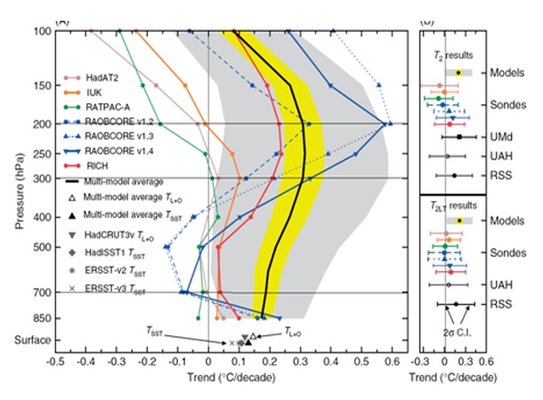
But S08 now claim that there are problems with the temperature data used in the CCSP report and call attention to “new observational estimates of surface and tropospheric temperature trends.” They state that “there is no longer a serious discrepancy between modelled and observed trends …” Their key graph [shown here as Fig. 4] conveys a (misleading) visual impression of an overlap between observations and GH model results.
I show here that no credible analysis supports the S08 claim of “consistency”: The “new observational estimates” are spurious. The GH model results used are inadequate for the intended purpose and may simply reflect chaotic and structural model uncertainties (which had been completely ignored by S08). My conclusion, therefore, is that the claimed “consistency of modeled and observed temperature trends” does not exist.
Section 1: Introduction
The principal issue here is the cause of warming observed in the past 30 years, the era of satellite temperature data: Is it mainly naturally caused or is it due to human-produced greenhouse (GH) gases? The question is of obvious importance since natural causes cannot be influenced by policies that limit emissions of GH gases, such as CO2. But resolving the question is a difficult scientific task. Natural causes are plausible; the climate has been warming and cooling for billions of years on many different time scales [see, e.g., Singer and Avery 2007; Loehle and Singer 2010]; there is no reason to assume that such natural climate fluctuations would suddenly cease. On the other hand, anthropogenic global warming (AGW) is also plausible, since the concentration of GH gases has been increasing due to human activities [see, e.g. IPCC 2007].
All parties seem to agree that both natural and anthropogenic factors have contributed to climate warming in the past 30 years; at issue is whether the human contribution has been preponderant and will grow in future — or whether it has been minor and will remain unimportant. All parties agree also on the proper methodology to distinguish between natural and human causes: It is the “fingerprint” method, which compares the pattern of temperature trends calculated from GH models with the pattern observed in the tropical atmosphere. By “pattern” we understand the distribution of temperature trends with latitude and altitude in the troposphere — with the tropical region being the crucial one.
This matter has been a contested issue since 1990 when early satellite results first showed no significant warming trend in the troposphere [Spencer and Christy 1990] – contrary to all expectations from GH models. The debate has involved the UN-sponsored IPCC (Intergovernmental Panel on Climate Change) –and more recently, the independent NIPCC (Nongovernmental Panel on Climate Change).
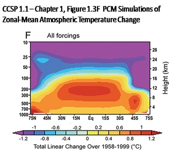
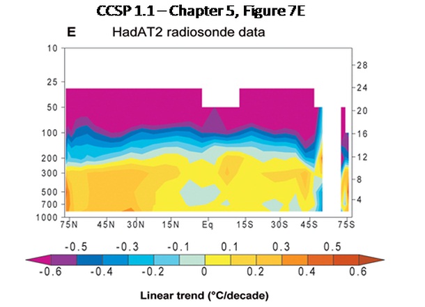
In 2004, Douglass, Pearson, and Singer [DPS 2004] carried out such a comparison using the best then-available data and models; they concluded that there was a real disparity and that the observations did not confirm GH models. Later, a major US government-funded effort, the Climate Change Science Program, arrived at essentially the same result. CCSP-SAP-1.1 [Karl et al 2006] found that while models predicted increasing trends with altitude in the tropical zone, observations actually showed a slight decrease (See Fig 1 and 2, which duplicate figures 1.3F and 5.7E of the CCSP report and figures 7 and 8 of the 2008 NIPCC report [NIPCC 2008].)
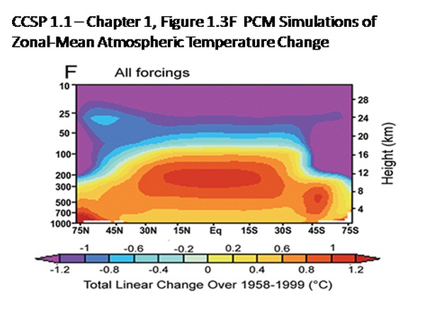
Fig 1: Model-predicted temperature trends versus latitude and altitude [this is figure 1.3F from CCSP 2006, p.25 and figure 7 from NIPCC 2008]. Note the increasing trends in the tropical mid-troposphere. All GH models show an amplification of temperature trend with altitude, up to about a factor 2, over the equator at 10 km. Also note: There is little variation with latitude in surface trends; NH is about the same as SH; but warming is expected in both polar regions – contrary to observations..
_____________________________________________________________________
Fig. 2: Observed temperature trends versus latitude and altitude [this is figure 5.7E from CCSP 2006, p.116 and figure 8 of NIPCC 2008]. Note the striking absence of any increasing trends in the tropical troposphere and the missing “hot spot” of Fig. 1.
___________________________________________________________________________
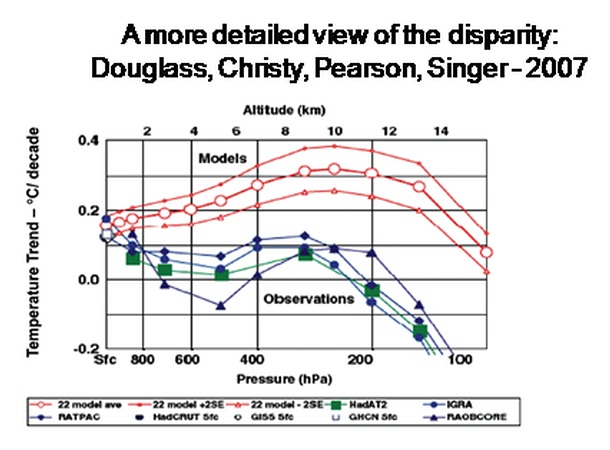
In 2007, Douglass, Christy, Pearson and Singer [hereinafter DCPS07] extended the DPS study by comparing in greater detail the published model-calculated trends with observed trends from balloons and satellites, in the tropical zone. They again concluded that the observations could not confirm the GH model results (Fig. 3). In 2008, a group of independent scientists — the Nongovernmental International Panel on Climate Change [NIPCC 2008] — published its summary report and simply compared the modeled (Fig. 1) and observed (Fig. 2) patterns of trends shown in the CCSP report.
NIPCC then stated the obvious logical conclusion – if one accepts the published CCSP results: Since GH models cannot explain the observed temperature trends in the tropical troposphere, then the warming of the past 30 years must be due predominantly to causes other than GH gases. In other words, the human contribution to the warming trend since 1979 is minor – a conclusion which is contrary to that of the IPCC [2007].
Fig. 3: Observed temperature trends versus latitude and altitude [this is figure 1 from DCPS 2007 and figure 10 of NIPCC 2008]. Note the disparity between (increasing) model trends and the decreasing observed trends in the tropical mid-troposphere.
___________________________________________________________
Deciding they could no longer ignore this issue, Santer and 16 coauthors [2008 – hereinafter S08] have critiqued the conclusions of both DCPS and NIPCC. They assert: [see Fig. 4]
(i) The observational data have changed; “new observational estimates” now show greater tropospheric warming trends.
(ii) The uncertainties of both models and data are greater than previously estimated.
(iii) Therefore, the discrepancy between models and atmospheric data in the tropics no longer exists.
In the present paper I address these issues and conclude that S08 have failed to demonstrate the claimed consistency – which is their main objection to DCPS and NIPCC.
Fig. 4: This is figure 6 from S08. Panel A shows tropospheric observed and modeled temperature trends vs. pressure-altitude (1979-1999; tropics 20oS-20oN). The RATPAC (NOAA) analyses agree well with Hadley and IUK, but are quite distinct from RICH and the RAOBCORE versions. The grey area shows model uncertainty according to S08; the yellow area represents the Standard Error of DCPS.
Panel B suggests good agreement of all observed and modeled tropospheric trend values (suitably weighted) with satellite data for both middle (T2 or MT ) and lower troposphere (T2LT or LT). See, however, the discussion in the text, which demonstrates that S08 did not use a suitable Discriminant.
_______________________________________________________________
Section 2: Conflicting sets of tropospheric temperature trends
Fig. 4 (which is figure 6 in S08) shows basically two sets of temperature trends. One set is derived from balloon-borne radiosondes, independently analyzed by the NOAA group and Hadley group; they agree fairly well with each other. This is the set used by DCPS07 and NIPCC.
The other set, showing drastically different trend values, especially in the upper troposphere, stems from the papers of Haimberger [2007 and “in press”]. S08 give no indication as to which of these two conflicting sets is credible, nor is there discussion of the cause of disagreement. The NOAA/Hadley results are based on direct observations, while the Haimberger results are derived from a reanalysis of temperature data, involving also a certain amount of modeling. Sakamoto and Christy [2009] have criticized his procedures.
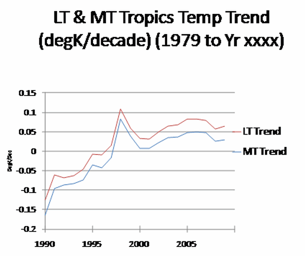
S08 claims that both the NOAA/Hadley data set and the Haimberger set are compatible with satellite data (see Fig. 4B, their figure 6B, and discussion). This indicates to me that their comparison is not a very sensitive one and that we need a better ‘Discriminant.’ In order to refine the comparison, I have therefore used the difference (of temperature trends) between the satellite results for the middle and lower troposphere. I have constructed a new ‘weight factor,’ which is the difference between the published ‘weight factors’ for MT and LT [Christy, private communication 2010]. I then apply this factor to each of the observed trend values. As can be seen from Fig. 5, temperature trends for both LT and MT are near zero, or even negative, up to 1997 – with the MT trend consistently less than LT’s. This result is clearly inconsistent with the “new datasets” introduced by S08 but supports the RATPAC-NOAA and HadAT2 datasets..
Fig 5: Temperature trend (K per decade) for the time period 1979 to end of year shown, for MSU-UAH-LT and MT data in the tropical region. Note absence of a positive trend until 1997 and the steep rise as a result of the 1998 super-El-Nino “warm spike.”
______________________________________________________________
Section 3: Climate models
In addition to the well-known problems of accurately defining various radiative forcings and simulating the relevant atmospheric, oceanic, and terrestrial processes, model problems include the lack of homogeneity, the basic issue of the chaotic nature of (non-linear) models, and the fundamental problems of ‘averaging’ a group of model results. This critique applies not only to S08, but also to the “multi-model ensemble averages” of the IPCC [2007], and to my earlier publication [DCPS 2007]. I try to show here that the estimates of uncertainty, indicated by the ‘grey area’ in Fig. 4A (figure 6A of S08), are an artifact. S08 considers them to be of a statistical nature; in reality, they reflect the chaotic nature of models.
3.1 Chaotic Variability
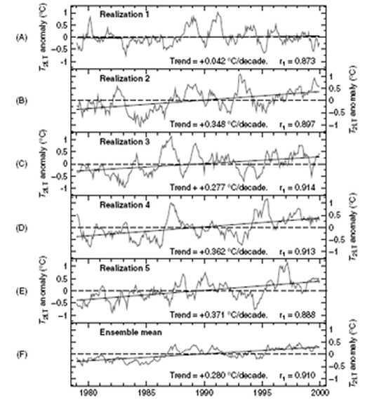
The chaotic nature of trends from climate models presents a fundamental problem. Successive runs of a model often lead to vastly different results. I show this in Fig 6, which is based on the five ‘runs’ of a particular GCM [Japan MRI model]. According to the results shown there, a single ‘run’ of a particular model can give trends spanning nearly a factor of ten. In actuality, had there been more than five runs, the range of trend values would have been even greater.
Fig. 6: Illustrating the chaotic nature of model trends, using the results of 5 runs (sometimes referred to as “realizations” or “simulations”) from 1979 to 1999 of a particular GCM (Japan MRI), as presented in figure 1 of S08. The OLS trends of the runs range from +0.042 to +0.371 (K per decade). (The range of trends is likely to be even larger if more runs had been displayed.) Selecting any 2 runs allows 10 possible means; there are 5 possibilities for the 4-run mean ensemble trend, and just one for a 5-run mean. It suggests convergence to a “true” trend, but as discussed in the text, one needs to show that the cumulative mean approaches an asymptotic value as the number of runs increases.
_________________________________________________________________________
However, as the number of runs increases, their cumulative average trend should converge to a single value. We don’t know where that is, but I have developed a synthetic approach that can increase the number of runs up to 25, and much greater; I then note when the cumulative trend approaches an asymptotic value [Singer 2010]. Of course, it becomes extremely expensive to increase the number of runs of an actual GCM; so in a practical sense one never carries out such an experiment. But it is intuitively obvious that a trend based on averaging a large number of runs should be less subject to chaotic variability and more reliable than a trend based on fewer or even just a single run.
This point becomes particularly relevant when we consider that the 22 models used by the IPCC have runs ranging from one up to nine [see Table II in DCPS07]. How then should one average these models? Shouldn’t we give greater weight to models that have more runs? The paper by S08 does not delve into this important matter; the dispersion shown in their figure 6 [grey area in Fig. 4] makes no allowance for the chaotic nature of models.
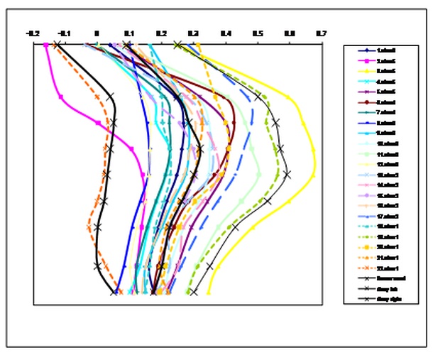
In Fig. 7, I plot trend values vs. altitude for all models. More or less as expected, the single-run models seem to show the widest dispersion. When I superimpose the limits of the ‘grey area of Fig. 4, I find that they show a similar dispersion One may conclude, therefore, that the model uncertainty, shown by the grey area, largely reflects chaotic variability – a factor completely ignored in the S08 analysis. If the IPCC compilation excluded single-run models, the grey area would shrink.
Fig. 7: Temperature trends (x-axis) and pressure-altitude (y-axis) for the twenty-two 20CEN models of IPCC shown in Table II of DCPS [2007]. Models #18 to 22 are single-run models and are shown here by short dashes. Models #13 to 17 are 2-run models and shown by long dashes. Models #1 to 12 have 3 or more runs and are shown by solid lines. The mean and the limits of the grey area of S08 (Fig, 5) are indicated by lines carrying X-crosses.
It is difficult to draw any firm conclusions from this graph, since the individual models also incorporate different structural uncertainties. But the single-run models show the widest dispersion, as expected, and also appear to cover the same area as the ‘grey area’ of S08.
3.2 The problem of averaging: over model runs or over model ensemble-means?
From a statistical point of view, one could consider each run as if it were an independent model – albeit using the same forcings and parameterizations. Therefore, one choice would be to average all of the runs (of all models), thereby giving greater weight to models with more runs and less weight to models with few runs. The alternative is to average first all of the runs of a particular model to obtain a “model ensemble-mean”, and then average these model means. But this latter method, chosen by S08, gives equal weight to each model irrespective of the number of runs – and therefore undue weight to “outliers.” More important even, it exaggerates the effects of chaotic variability.
This problem has not been successfully tackled. Yet the S08 claim of ‘consistency’ hinges on the degree of agreement between observed and modeled trends. By ignoring the chaotic and structural uncertainties, the analysis by S08 has served to increase the uncertainties in the model trends, and thus any ‘overlap’ with observed trend values: (Compared to this, the issue of auto-correlation discussed in S08 is relatively unimportant.)
Section 4: Conclusions
I conclude that the S08 claim that observed and modeled trends are “consistent” is invalid. Specifically, the “new observational evidence” presented in S08 does not hold up to scrutiny. The claimed uncertainties of the modeled temperature trends, although seemingly supported by elaborate statistical analysis, fail to consider the more important chaotic and structural uncertainties. I hope that my critique will serve to avoid the kind of disastrous mistake that led to the 1997 Kyoto Protocol.
**********************************************
References
Douglass DH, Pearson BD, Singer SF. 2004. Altitude dependence of atmospheric temperature trends: Climate models versus observations. Geophysical Research Letters 31: L13208, Doi:10.1029/2004/GL020103.
Douglass DH, Christy JR, Pearson BD, Singer SF. DCPS 2007. A comparison of tropical temperature trends with model predictions. International Journal of Climatology 27: Doi:10.1002/joc.1651. In printed form: IJC 28:1693-1701 (2008)
Free, M.; Seidel, D.J.; Angell, J.K.; Lanzante, J.; Durre, I.; Peterson, T.C. Radiosonde Atmospheric Temperature Products for Assessing Climate (RATPAC) 2005: A new data set of large-area anomaly time series, J. Geophys. Res. 110, doi:10.1029/2005JD006169.
Haimberger L. 2007. Homogenization of radiosonde temperature time series using innovation statistics. Journal of Climate 20: 1377–1403.
IPCC AR4. Climate Change 2007: The Physical Science Basis. Contribution of Working Group I to the Fourth Assessment Report of the Intergovernmental Panel on Climate Change; Solomon, S., Qin, D., Manning, M., Chen, Z., Marquis, M., Avery, K.B., Tignor, M., Miller, H.L., Eds.; Cambridge University Press: Cambridge, UK and New York, NY.
Karl, T.R.; Hassol, S.J.; Miller, C.D.; Murray, W.L. Temperature Trends in the Lower Atmosphere: Steps for Understanding and Reconciling Differences; U.S. Climate Change Science Program Synthesis and Assessment Product 1.1(CCSP-SAP-1.1 2006); Washington, DC..
Loehle C and SF Singer. 2010. Holocene temperature records show millennial-scale periodicity. Can J Earth Sci 47:1327-1336
Mitchell JFB, et al. 2001. Detection of climate change and attribution of causes. In Climate Change 2001: The Scientific Basis, Contribution of Working Group I to the Third Assessment Report of the Intergovernmental Panel on Climate Change, Mitchell JFB, Karoly DJ, Hegerl GC, Zwiers FW, Allen MR, Marengo J (eds). Cambridge University Press: Cambridge, New York; 881.
NAS-National Research Council 2000.. Reconciling Observations of Global Temperature Change. National Academy Press, Washington DC.
Sakamoto, M.; Christy, J.R. 2009. The influences of TOVS radiance assimilation on temperature and moisture tendencies in JRA-25 and ERA-40. J. Atmos. Ocean. Tech., 26, 1435.
Santer BD, Penner JE, Thorne PW. 2006. How well can the observed vertical temperature changes be reconciled with our understanding of the causes of these changes? In Temperature Trends in the Lower Atmosphere: Steps for Understanding and Reconciling Differences, Karl TR, Hassol SJ, Miller CD, Murray WL (eds). A Report by the U.S. Climate Change Science Program and the Subcommittee on Global Change Research, Washington DC.
Santer, B.D.; Thorne, P.W.; Haimberger, L.; Taylor, K.E.; Wigley, T.M.L.; Lanzante, J.R.; Solomon, S.; Free, M.; Gleckler, P.J.; Jones, P.D.; Karl, T.R.; Klein, S.A.; Mears, C.; Nychka, D.; Schmidt, G.A.; Sherwood, S.C.; Wentz, F.J. S08. Consistency of modelled and observed temperature trends in the tropical troposphere. Int. J. Climatol. 2008, doi:1002/joc.1756.
Singer, S.F. 2000: Climate Policy – From Rio to Kyoto A Political Issue for 2000 -and Beyond. Essays in Public Policy No. 102. Hoover Institution, Stanford, California.
Singer, S.F., D.T. Avery, 2007: Unstoppable Global Warming: Every 1,500 Years. Rowman & Littlefield Publishers, Inc. Lanham, MD
Singer SF. 2008. Nature, Not Human Activity, Rules the Climate: Summary for Policymakers of the Report of the Nongovernmental International Panel on Climate Change (NIPCC), Heartland Institute: Chicago, IL.
Singer SF. 2010. Overcoming chaotic variability of climate models (submitted for publication)
Spencer RW and JR Christy 1990. Precise monitoring of global temperature trends from satellites. Science 247: 1558–1562.
Thorne, P.W.; Parker, D.E.; Santer, B.D.; McCarthy, M.P.; Sexton, D.M.H.; Webb, M.J.; Murphy, J.M.; Collins, M.; Titchner, H.A.; Jones, G.S. HadAT2 2007. Tropical vertical temperature trends. Geophys. Res. Lett. 34, doi:10;1029/2007GL029875.

